ECMWF model output for the SHEBA column
Chris Bretherton, University of Washington
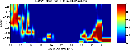
As a member of the FIRE Science Team, ECMWF generously provided
hourly forecast model output for the SHEBA column to the FIRE/SHEBA
Science Team, including many non-standard fields (such as radiative
fluxes, surface temperature and winds, and vertical distributions of
cloud and ice water and precipitation) at the full 31-level vertical
resolution of the model. The model output is taken from 12-35 hour
forecasts of the ECMWF operational model, which were sent daily to
the University of Washington from 22 Oct 97-30 Sept 98. The
twice-daily soundings and routine surface observations of pressure,
wind, temperature, humidity from the ice camp were assimilated into
the model to help initialize each daily forecast cycle. Statistics
for Nov 97- Jan 98 suggest that roughly 85% of the soundings reached
ECMWF and entered the analysis; click here
for a technical discussion of model bias and error statistics at SHEBA over
this period. Overall,
this discussion suggests that the model wind and temperature fields
are quite close to the sounding measurements. However, other fields
are generated by the model itself with little direct constraint from
SHEBA observations, and MUST NOT BE REGARDED AS OBSERVATIONS. One
can see sharp, usually small, jumps at periodic intervals
representing the effects of corrected initial conditions on the
forecasts.
The model output has been improved (18 Feb 00) from its original
version through the considerable efforts of Chris Jakob and lots of
cycles of ECMWF's computers, by removing large position errors that
existed in the original dataset and also by using the same forecast
model version (13R4) to produce the equivalent of a 'reanalysis'. It
is now for the grid column nearest to the exact (time-varying) ice
camp location, which is at all times less than 50 km away from the ice
camp location.
The ECMWF model physics are far too complex to fully describe here. In
summary, they include prognostic equations for cloud fraction, liquid
water, ice, and precipitation, a convection scheme that has a separate
treatment of stratocumulus cloud which only occupy a single grid level
that can be active in the summertime Arctic boundary layer,
first-order closure for turbulence including stability corrections, a
state-of-the-art radiation scheme incorporating cloud effects, and a
single layer
sea ice scheme in which the thickness and extent of sea ice are
specified, but the ice slab temperature interacts with the atmosphere.
We encourage all of you to use and reality-check the
ECMWF output vs. SHEBA observations that you
may have. Two papers describing aspects of this comparison have been
submitted to JGR:
-
Beesley, T. A., C. S. Bretherton, C. Jakob, E. L Andreas,
J. M. Intrieri, and T. A. Uttal, 2000: A comparison of the ECMWF
forecast model with observations at SHEBA, J. Geophys. Res.,
submitted 6/99, revised and accepted 12/99.
- Bretherton,
C. S., S. R. de Roode, and C. Jakob, 2000: A comparison of the
ECMWF forecast model with observations over the annual cycle at
SHEBA. J. Geophys. Res., submitted 12/99.
If you make use of this dataset, please acknowledge ECMWF as follows:
'We thank Christian Jakob and his coworkers at ECMWF for producing the
ECMWF column dataset for SHEBA.'
Here, we describe what model fields are being archived
here, we provide a suite of plots which summarize
the model output, and we describe how FIRE/SHEBA
Science Team members can access it. My contribution to this work has been
sponsored by NASA as part of the FIRE program under grants
NAG1-1711 and NAG1-2072. Chris Jakob and Martin Miller of ECMWF have been
instrumental in making this extraordinary suite of model outputs
available to our community. Chris Jakob has an even more extensive
set of model diagnostics archived at ECMWF, so if you do not see what
you need, you might want to email him at paj@ecmwf.int .
Model Fields Archived
Basic fields
- pressure (Pa)
- zonal wind component (m/s)
- meridional wind component (m/s)
- temperature (K)
- specific humidity (kg/kg)
- specific cloud liquid water content (kg/kg)
- specific cloud ice content (kg/kg)
- cloud fraction (percent/100.)
- relative humidity (percent/100.)
- omega=vertical velocity in pressure coordinates (Pa/s)
Fluxes
- net shortwave flux (W/m2)
- net longwave flux (W/m2)
- sensible heat flux (W/m2)
- turbulent moisture flux (kg/kg * kg/(m2*s))
- x turbulent momentum flux (= x wind stress, at bottom level) (kg/(m-s))
- y turbulent momentum flux (= y wind stress, at bottom level) (kg/(m-s))
- turbulent moisture flux (kg/kg * kg/(m2*s))
- convective rain flux (kg/(m2*s) = mm/s)
- convective snow flux (mm/s)
- large-scale rain flux (mm/s)
- large-scale snow flux (mm/s)
Tendencies
- dudt_total (m/s2)
- dudt_nonadiabatic (m/s2)
- dvdt_total (m/s2)
- dvdt_nonadiabatic (m/s2)
- dTdt_total (K/s)
- dTdt_nonadiabatic (K/s)
- dqdt_total (1/s)
- dqdt_nonadiabatic (1/s)
Surface variables
- surface pressure (Pa)
- 2-m temperature (K)
- 2-m specific humidity (kg/kg)
- 10-m wind u component (m/s)
- 10-m wind v component (m/s)
- skin temperature (K)
- surface roughness length (m)
- surface roughness length for heat (m)
- surface albedo (%/100.)
- downward surface solar radiation (W/m2)
- downward surface thermal radiation (W/m2)
Based on ECMWF output starting 97/10/22
| Variables |
Oct 97 |
Nov 97 |
Dec 97 |
Jan 98 |
Feb 98 |
Mar 98 |
Apr 98 |
May 98 |
Jun 98 |
Jul 98 |
Aug 98 |
Sep 98 |
|
|
| 2 m temperature, skin temperature |
gif,
eps |
gif,
eps |
gif,
eps |
gif,
eps |
gif,
eps |
gif,
eps |
gif,
eps |
gif,
eps |
gif,
eps |
gif,
eps |
gif,
eps |
gif,
eps |
| 10 m u and v |
gif,
eps |
gif,
eps |
gif,
eps |
gif,
eps |
gif,
eps |
gif,
eps |
gif,
eps |
gif,
eps |
gif,
eps |
gif,
eps |
gif,
eps |
gif,
eps |
| Surface downwelling LW, SW |
gif,
eps |
gif,
eps |
gif,
eps |
gif,
eps |
gif,
eps |
gif,
eps |
gif,
eps |
gif,
eps |
gif,
eps |
gif,
eps |
gif,
eps |
gif,
eps |
| TOA, surface net LW radiation |
gif,
eps |
gif,
eps |
gif,
eps |
gif,
eps |
gif,
eps |
gif,
eps |
gif,
eps |
gif,
eps |
gif,
eps |
gif,
eps |
gif,
eps |
gif,
eps |
| TOA, surface net SW radiation |
gif,
eps |
gif,
eps |
gif,
eps |
gif,
eps |
gif,
eps |
gif,
eps |
gif,
eps |
gif,
eps |
gif,
eps |
gif,
eps |
gif,
eps |
gif,
eps |
| Surface energy fluxes |
gif,
eps |
gif,
eps |
gif,
eps |
gif,
eps |
gif,
eps |
gif,
eps |
gif,
eps |
gif,
eps |
gif,
eps |
gif,
eps |
gif,
eps |
gif,
eps |
Surface moisture fluxes |
gif,
eps |
gif,
eps |
gif,
eps |
gif,
eps |
gif,
eps |
gif,
eps |
gif,
eps |
gif,
eps |
gif,
eps |
gif,
eps |
gif,
eps |
gif,
eps |
| Wind stress |
gif,
eps |
gif,
eps |
gif,
eps |
gif,
eps |
gif,
eps |
gif,
eps |
gif,
eps |
gif,
eps |
gif,
eps |
gif,
eps |
gif,
eps |
gif,
eps |
| ECMWF column and actual ice camp lat/lon |
gif,
eps |
gif,
eps |
gif,
eps |
gif,
eps |
gif,
eps |
gif,
eps |
gif,
eps |
gif,
eps |
gif,
eps |
gif,
eps |
gif,
eps |
gif,
eps |
| Mean monthly temperature profile |
gif,
eps |
gif,
eps |
gif,
eps |
gif,
eps |
gif,
eps |
gif,
eps |
gif,
eps |
gif,
eps |
gif,
eps |
gif,
eps |
gif,
eps |
gif,
eps |
| Mean monthly RH and cloud frac profiles |
gif,
eps |
gif,
eps |
gif,
eps |
gif,
eps |
gif,
eps |
gif,
eps |
gif,
eps |
gif,
eps |
gif,
eps |
gif,
eps |
gif,
eps |
gif,
eps |
| Mean liquid and ice water profiles |
gif,
eps |
gif,
eps |
gif,
eps |
gif,
eps |
gif,
eps |
gif,
eps |
gif,
eps |
gif,
eps |
gif,
eps |
gif,
eps |
gif,
eps |
gif,
eps |
| Temperature time-height section |
gif,
eps |
gif,
eps |
gif,
eps |
gif,
eps |
gif,
eps |
gif,
eps |
gif,
eps |
gif,
eps |
gif,
eps |
gif,
eps |
gif,
eps |
gif,
eps |
| u, v time-height sections |
gif,
eps |
gif,
eps |
gif,
eps |
gif,
eps |
gif,
eps |
gif,
eps |
gif,
eps |
gif,
eps |
gif,
eps |
gif,
eps |
gif,
eps |
gif,
eps |
| Vert. motion and rel. hum. |
gif,
eps |
gif,
eps |
gif,
eps |
gif,
eps |
gif,
eps |
gif,
eps |
gif,
eps |
gif,
eps |
gif,
eps |
gif,
eps |
gif,
eps |
gif,
eps |
| Cloud fraction |
gif,
eps |
gif,
eps |
gif,
eps |
gif,
eps |
gif,
eps |
gif,
eps |
gif,
eps |
gif,
eps |
gif,
eps |
gif,
eps |
gif,
eps |
gif,
eps |
| Cloud water and ice |
gif,
eps |
gif,
eps |
gif,
eps |
gif,
eps |
gif,
eps |
gif,
eps |
gif,
eps |
gif,
eps |
gif,
eps |
gif,
eps |
gif,
eps |
gif,
eps |
| Adiabatic, nonad. dTdt |
gif,
eps |
gif,
eps |
gif,
eps |
gif,
eps |
gif,
eps |
gif,
eps |
gif,
eps |
gif,
eps |
gif,
eps |
gif,
eps |
gif,
eps |
gif,
eps |
| Adiabatic, nonad. dqdt |
gif,
eps |
gif,
eps |
gif,
eps |
gif,
eps |
gif,
eps |
gif,
eps |
gif,
eps |
gif,
eps |
gif,
eps |
gif,
eps |
gif,
eps |
gif,
eps |
| Mean ad, nonad dTdt, dqdt |
gif,
eps |
gif,
eps |
gif,
eps |
gif,
eps |
gif,
eps |
gif,
eps |
gif,
eps |
gif,
eps |
gif,
eps |
gif,
eps |
gif,
eps |
gif,
eps |
|
|
The ECMWF model output for each day is stored as a compressed unix tar
file SHEBA_yymmdd.tar.gz. Here yy = 97 or 98 is the year, mm = 01-12
is the month, and dd is the day. All of these files can be downloaded
from the anonymous ftp directory pub/breth/SHEBA
on eos.atmos.washington.edu. The help file readme_ARM_ddh_sheba in
this directory explains what to do with these daily files and what
output is included.
I have also accumulated this output in a netcdf file for the entire
period 22 Oct 97-30 Sep 98, which is a considerably more convenient
way to access the data, especially if you use a graphics program that
has a good interface to netcdf (such as matlab or NCAR graphics). The
plots above were created with matlab using the netcdf file. The
advantage of this format is that it is very easy to extract the subset
of data that you wish to look at without having to parse the rest, and
that the format is self-documenting so that it is easy to figure out
what data is included and by what names. This netcdf
dataset (60 MB!) is for use by any FIRE/SHEBA Science Team
member.
Chris Bretherton <breth@atmos.washington.edu>


