Cross-spectral analysis Nino3.4 vs. North Pacific Index

Contents

Plot sea-surface temperature and NPI anomalies

  load SSTA;   % loads decimal year yr and Nino3.4 SSTA [C].
  N = length(yr);  % Number of monthly samples
  Nyr = round(N/12);  % Number of years in data record

  NPdat = load('NPindex_monthly.txt');
  yyyymm = NPdat(:,1);
  post1950 = (yyyymm>195000);
  pre2013 = (yyyymm<201300);
  NPI = NPdat(post1950&pre2013,2);  % 63 years of monthly data,
                                    % 1950-2012, like SSTA
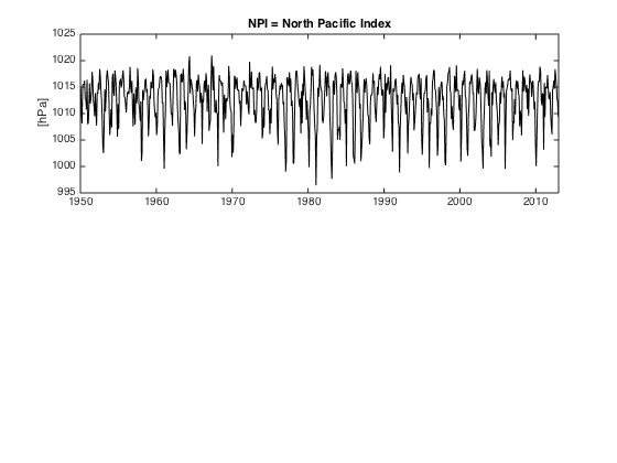
  figure(1)
  clf

  subplot(2,1,1)
  plot(yr,NPI,'k')
  ylabel('[hPa]')
  title('NPI = North Pacific Index')
  xlim([1950 2013])

  % Remove mean seasonal cycle

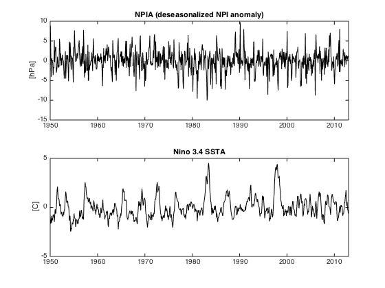
Deseasonalize to get NPIA; compare with Nino 3.4 SSTA

  NPIhat = fft(NPI);
  NPIAhat = NPIhat;
  filtindex = [1 + (0:3)*Nyr N+1 - (1:3)*Nyr];
  NPIAhat(filtindex) = 0;
  NPIA = real(ifft(NPIAhat));

  subplot(2,1,1)
  plot(yr,NPIA,'k')
  ylabel('[hPa]')
  title('NPIA (deseasonalized NPI anomaly)')
  xlim([1950 2013])

  subplot(2,1,2)
  plot(yr,SSTA,'k')
  ylabel('[C]')
  title('Nino 3.4 SSTA')
  xlim([1950 2013])
  ylim([-5 5])

Are SSTA and NPIA correlated?

  R = corrcoef(NPIA,SSTA);
  R_SSTA_NPIA = R(1,2)

% There is some anticorrelation between Nino3.4 SSTA and NPI

R_SSTA_NPIA =

   -0.1707

One-sided spectra/cross spectra

Nwyr = 20;  % Window length [yr]
rate = 12;  % Sampling rate [1/yr] (1/month = 12/yr)
Nw = Nwyr*rate; % Window length in months
df = 1/Nwyr;  % Frequency increment for windowed spectra [1/yr]
fn = rate/2;  % Nyquist frequency [1/yr]

[Pxy,f]=cpsd(SSTA,NPIA,hann(Nw),Nw/2,Nw,rate);
[Pxx,f]=pwelch(SSTA,hann(Nw),Nw/2,Nw,rate);
[Pyy,f]=pwelch(NPIA,hann(Nw),Nw/2,Nw,rate);
Cohxy = Pxy./sqrt(Pxx.*Pyy);

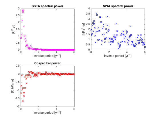
Plot the windowed power spectra of SSTA and NPIA and their cospectrum

figure(2)
clf

subplot(221)
plot(f,real(Pxx),'mx')
xlim([0 fn])
xlabel('Inverse period [yr^{-1}]')
ylabel('[C^2 yr]')
title('SSTA spectral power')

subplot(222)
plot(f,real(Pyy),'bx')
xlim([0 fn])
xlabel('Inverse period [yr^{-1}]')
ylabel('[hPa^2 yr]')
title('NPIA spectral power')

subplot(223)
plot(f,real(Pxy),'rx',[0 max(f)],[0 0],'k--')
xlim([0 fn])
xlabel('Inverse period [yr^{-1}]')
ylabel('[C hPa yr]')
title('Cospectral power')

Frequency partitioning of covariance

% Show near-equality of covariance and the frequency integral
% of the windowed cospectral power real(Pxy)

cov12 = cov(SSTA,NPIA);
cov_SSTA_NPIA = cov12(1,2)
covWinFreqIntegral_SSTA_NPIA =sum(real(Pxy)*df)

cov_SSTA_NPIA =

   -0.5093


covWinFreqIntegral_SSTA_NPIA =

   -0.5169

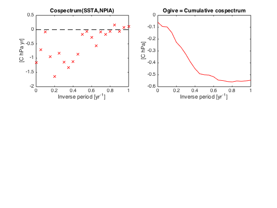
Replot cospectrum including only subannual frequencies; plot ogive

figure(3)
clf

subplot(221)
plot(f,real(Pxy),'rx',[0 max(f)],[0 0],'k--')
xlim([0 1])
xlabel('Inverse period [yr^{-1}]')
ylabel(' [C hPa yr] ')
title('Cospectrum(SSTA,NPIA)')

subplot(222)
plot(f,cumsum(Pxy*df),'r-')
xlim([0 1])
xlabel('Inverse period [yr^{-1}]')
ylabel('[C hPa]')
title('Ogive = Cumulative cospectrum')

% The cospectrum of SSTA and NPIA is generally negative (anti-correlation)
% across subannual frequencies.
% The ogive shows how this accumulates to produce negative covariance.

Warning: Imaginary parts of complex X and/or Y arguments ignored 

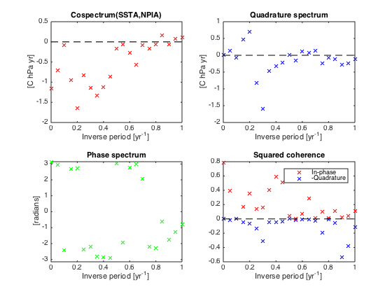
Quadrature spectrum, phase and magnitude-squared coherence

subplot(222)
plot(f,imag(Pxy),'bx',[0 max(f)],[0 0],'k--')
xlim([0 1])
xlabel('Inverse period [yr^{-1}]')
ylabel(' [C hPa yr] ')
title('Quadrature spectrum')

subplot(223)
plot(f,angle(Pxy),'gx')
xlim([0 1])
ylim([-pi pi])
xlabel('Inverse period [yr^{-1}]')
ylabel(' [radians] ')
title('Phase spectrum')

subplot(224)
plot(f,real(Cohxy).^2,'rx',f,-imag(Cohxy).^2,'bx',[0 max(f)],[0 0],'k--')
xlim([0 1])
xlabel('Inverse period [yr^{-1}]')
title('Squared coherence')
legend('In-phase','-Quadrature')

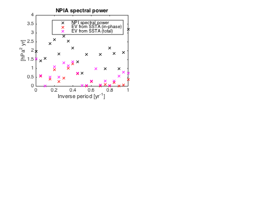
Variance of NPI explained by SSTA

figure(4)
clf

subplot(221)
plot(f,real(Pyy),'kx')
xlim([0 1])
xlabel('Inverse period [yr^{-1}]')
ylabel('[hPa^2 yr]')
title('NPIA spectral power')
hold on
plot(f,real(Pyy).*real(Cohxy).^2,'rx',f,real(Pyy).*abs(Cohxy).^2,'mx')
legend('NPI spectral power','EV from SSTA (in-phase)','EV from SSTA (total)')
hold off

% Most of the Nino-explained variance in NPI is at periods > 2 yr,
% and most is due to in-phase covariability.

Published with MATLAB® R2014b