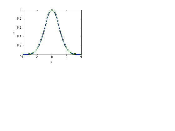
DFT example using u(x) = exp(-x^2/2)
Contents
Define parameters and functions
dx = 2^-3;
L = 2^3;
N = round(L/dx);
x = -L/2 + (0:(N-1))*dx;
u = exp(-0.5*x.^2);
clf
figure(1)
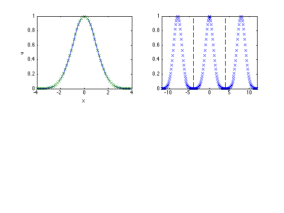
Plot u
subplot(2,2,1)
plot(x,u,'-',x,u,'x')
xlabel('x')
ylabel('u')
Plot periodic extension of u
subplot(2,2,2)
plot([x-L x x+L],[u u u],'x',...
    [-L/2 -L/2],[0 1],'k--',[L/2 L/2],[0 1],'k--')
xlim([-3*L/2 3*L/2])
Plot power spectrum of u
subplot(2,2,3)
uhat = fft(u);
upow = (abs(uhat)/N).^2;
m = 1:N;
plot(m,upow,'x')
xlabel('m')
xlim([0 N])
ylabel('(|uhat|/N)^2')

Replot using semilogy
subplot(2,2,3)
semilogy(m,upow,'x')
xlabel('m')
xlim([0 N])
ylabel('(|uhat|/N)^2')
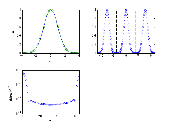
Replot using the corresponding harmonics
M = [0:(N/2 - 1) -N/2:-1];
semilogy(M,upow,'x')
xlabel('M')
xlim([-N/2 N/2])
ylabel('(|uhat|/N)^2')

Parseval theorem
sum_upow = sum(upow)
uvar = sum(u.^2)/N
gauss_integral = sqrt(pi)
uex_var = gauss_integral/L
sum_upow =

    0.2216


uvar =

    0.2216


gauss_integral =

    1.7725


uex_var =

    0.2216
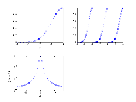
Now do DFT with [-L/2 0]
Nh = N/2;
xh = x(1:Nh);
uh = u(1:Nh);

figure(2)

subplot(2,2,1)
plot(xh,uh,'x')
xlabel('x')
ylabel('u')

subplot(2,2,2)
plot([xh-L/2 xh xh+L/2],[uh uh uh],'x',...
    [0 0],[0 1],'k--',[L/2 L/2],[0 1],'k--')
xlim([-L L/2])

subplot(2,2,3)
uhhat = fft(uh);
uhpow = (abs(uhhat)/Nh).^2;
m = 1:Nh;
M = [0:(Nh/2-1) -Nh/2:-1];
semilogy(M,uhpow,'x')
xlabel('M')
xlim([-Nh/2 Nh/2])
ylabel('(|uhhat|/Nh)^2')