Maximum covariance analysis (MCA) example

Analyze how temperature across the U.S. covaries
with tropical Pacific sea-surface temperature anomalies

Contents

Load data

% Load land temperature data

clear
load USTA;  % US monthly temperature anomaly on 5x5 degree grid
            % over U.S (NOAA GHCN3), Jan. 1970-Dec. 2002

% Define other useful parameters for USTA dataset

latUS = lat;
latmaxUS = latUS(1);
latminUS = latUS(end);
nlatUS = length(latUS);

lonUS = lon;
lonminUS = lonUS(1);
lonmaxUS = lonUS(end);
nlonUS = length(lonUS);
nsUS = nlatUS*nlonUS;

nyear = length(year);
nt = 12*nyear;

TAland = reshape(TA,nsUS,nt);
landUS = land(:);
TAland = TAland(landUS,:); % Only keep land points

% Load, de-time-mean and de-nan the SST data

load SSTPac
landPac = land;
SST = PSSTA(~landPac,:);
SST = SST - mean(SST,2)*ones(1,nt);  % Remove any residual time-mean at each location.
latmaxPac = latmax;
latminPac = latmin;
lonmaxPac = lonmax;
lonminPac = lonmin;
nlatPac = (latmaxPac - latminPac)/2 + 1;
nlonPac = (lonmaxPac - lonminPac)/2 + 1;
nsPac = nlatPac*nlonPac; % Number of Pacific spatial gridpoints

SVD of covariance matrix

Cxy = SST*TAland'/(nt-1);
[U,Sigma,V] = svd(Cxy,0);  % Always use 0 argument (economy SVD option) to
                       % prevent possible massive unneeded computation.
s = diag(Sigma);

scf = s.^2/sum(s.^2);

figure(1)
clf
plot(cumsum(scf),'x')  % Cumulative fraction of squared covariance explained
xlabel('SVD mode')
ylabel('Cumulative squared covariance fraction')

% Leading 2 modes each explain about 40% of squared covariance
% Leading 3 modes together explain almost 95% of squared covariance

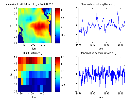
Plot the leading MCA spatial left/right pattern and time series

Normalize by standardizing the time series, so patterns correspond to
a 1 standard-deviation variation in a1 or b1
Also, reverse the sign of U1 and V1 so El Nino SSTA is a positive a1.

Uall = nan(nsPac,1);
Uall(~landPac,:) = -U(:,1);
U1 = reshape(Uall(:,1),nlonPac,nlatPac);  % Turn column of U into lat/lon mx

% Left time series

subplot(2,2,2)
a1 = (-U(:,1))'*SST;
plot(yd,a1/std(a1))
xlabel('year')
xlim([1970 2003])
title('Standardized left amplitude a_1')

% Left pattern (normalized by multiplying by std(a1)

subplot(2,2,1)
image([lonminPac lonmaxPac],[latminPac latmaxPac],U1'*std(a1),'CDataMapping','scaled')
xlabel('lon')
ylabel('lat')
title(['Normalized Left Pattern U_1; scf = ' num2str(scf(1))])
axis xy
colorbar

Vall = nan(nsUS,1);
Vall(landUS,:) = -V(:,1);  % Put the first two patterns into the land points
                            % of the two columns of Uall. Ocean points = nan
V1 = reshape(Vall(:,1),nlatUS,nlonUS); % Turn column V into lat/lon mx

% Right time series
subplot(2,2,4)
b1 = (-V(:,1))'*TAland;
plot(yd,b1/std(b1))
xlabel('year')
xlim([1970 2003])
title('Standardized right amplitude b_1')

subplot(2,2,3)
image([lonminUS lonmaxUS],[latmaxUS latminUS],V1*std(b1),'CDataMapping','scaled')
xlabel('lon')
ylabel('lat')
title('Right Pattern V_1')
axis xy
colorbar

% Similar to the Nino 3.4 regression of US temperature anomaly with a
% little warming trend mixed in.

sigma1 = s(1)
cov_a1_b1 = a1*b1'/(nt-1)  % Equals first singular value s(1)
R1 = corrcoef(a1,b1);
corrcoef_a1_b1 = R1(2,1)   % Correlation coeff > 0 but not too high due to
                           % noisiness in U. S. temperature time series.

sigma1 =

   21.6023


cov_a1_b1 =

   21.6023


corrcoef_a1_b1 =

    0.2597

Published with MATLAB® R2012b