PCA of tropical Pacific monthly SSTA dataset (Jan 1970- Dec 2002)
Contents
- Load data
- Define dimensions
- Graphically time-step through it
- Do PCA using svd
- A more efficient way to compute leading SVD modes
- Extract leading space and time modes of variability
- Renormalize patterns and time series for easier interpretation
- Linearity
- Look if PDF of PC1 is multimodal (shows clustering)
- Now add plots for mode 2
Load data
clear
load SSTPac
whos
  Name           Size               Bytes  Class      Attributes

  PSSTA       2520x396            7983360  double
  land        2520x1                 2520  logical
  lat         2520x1                20160  double
  latmax         1x1                    8  double
  latmin         1x1                    8  double
  lon         2520x1                20160  double
  lonmax         1x1                    8  double
  lonmin         1x1                    8  double
  yd             1x396               3168  double
Define dimensions
nt = length(yd);
nlat = (latmax - latmin)/2 + 1;
nlon = (lonmax - lonmin)/2 + 1;
ns = nlat*nlon; % Number of spatial gridpoints
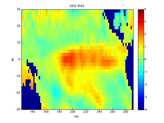
Graphically time-step through it
figure(1)
clf
for i = 1:nt
  PSSTAi = reshape(PSSTA(:,i),nlon,nlat);
  image([lonmin lonmax],[latmin latmax],PSSTAi','CDataMapping','scaled')
  xlabel('lon')
  ylabel('lat')
  axis xy
  title(num2str(yd(i)))
  caxis([-4 4])
  colorbar
  getframe; % Used to force 'run' mode to spit out updated plot
end
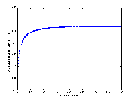
Do PCA using svd
% Remove the land points before doing analysis to avoid issues with NaNs.

SST = PSSTA(~land,:);

% Remove any residual time-mean at each location.

SST = SST - mean(SST,2)*ones(1,nt);

[U,Sigma,V] = svd(SST,0);  % Always use 0 argument (economy SVD option) to
                       % prevent possible massive unneeded computation.
sizeU=size(U)  % Since ns>nt this only gives the first nt columns of U, which is
         % thus nt x nt
         % Other columns would correspond to zero singular values
sizeSig=size(Sigma)  % Also, we only get the first nt rows of S, which is thus nt x nt.
sizeV=size(V)  % This will be the full nt x nt matrix in this case.
s = diag(Sigma); % Vector of singular values

% Plot cumulative variance explained by first k modes

normsqS = sum(s.^2)         % Show sum of SVs equals
normsqSST = sum(SST(:).^2)  % sum of squares of entries of SST

plot(cumsum(s.^2)/(ns*nt),'x')  % Divide by number of entries in SST
                                % to plot a cumulative mean square variance
xlabel('Number of modes')
ylabel('Cumulative explained variance [C^2]')

varfrac1 = s(1)^2/normsqS   % Fraction of variance explained by modes 1&2
varfrac2 = s(2)^2/normsqS
sizeU =

        2261         396


sizeSig =

   396   396


sizeV =

   396   396


normsqS =

   3.7026e+05


normsqSST =

   3.7026e+05


varfrac1 =

    0.3892


varfrac2 =

    0.0926
A more efficient way to compute leading SVD modes
% Note:  For efficiency we can just compute the first two SVD modes as
% follows - now U is ns x 2, V is nt by 2, and S is diagonal 2x2.

[U,Sigma,V] = svds(SST,2);
sizeU=size(U)
sizeSig=size(Sigma)
sizeV=size(V)
sizeU =

        2261           2


sizeSig =

     2     2


sizeV =

   396     2
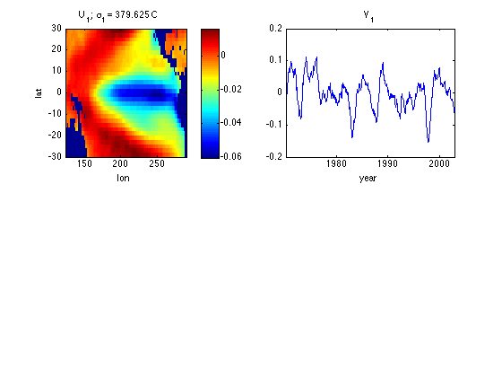
Extract leading space and time modes of variability
This code will work whether svd or svds was used to find U and V Columns of U give spatial patterns Columns of V give the corresponding time series Note each column of U, V has 2-norm of 1.
Uall = nan(ns,size(U,2));
Uall(~land,:) = U;

U1 = reshape(Uall(:,1),nlon,nlat);  % Turn column of U into a lat/lon
                                    % matrix including nan's at land points
V1 = V(:,1);

subplot(2,2,1)
image([lonmin lonmax],[latmin latmax],U1','CDataMapping','scaled')
xlabel('lon')
ylabel('lat')
title(['U_1; \sigma_1 = ' num2str(s(1)) ' C'])
axis xy
colorbar

subplot(2,2,2)
plot(yd,V1)
xlabel('year')
xlim([yd(1) yd(end)])
title('V_1')
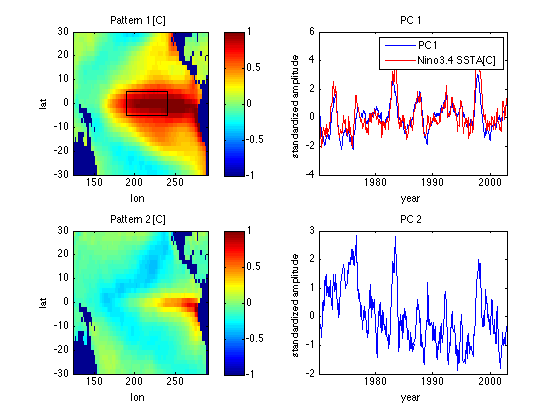
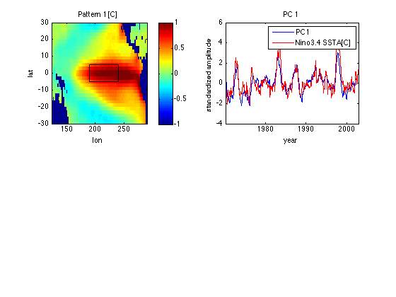
Renormalize patterns and time series for easier interpretation
PC1 = -V1*sqrt(nt-1);        % PC1 = V1 renormalized to have std=1
Ut1 = -U1*s(1)/sqrt(nt-1);   % Ut1 = SST for PC1 = +1 std.
                             % With 20-20 hindsight we also flip signs
                             % of pattern and PC (which are ambiguous)
                             % to match normal conventions.
subplot(2,2,1)
image([lonmin lonmax],[latmin latmax],Ut1','CDataMapping','scaled')
xlabel('lon')
ylabel('lat')
title('Pattern 1 [C]')
caxis([-1 1])
axis xy
colorbar

hold on

% Add Nino3.4 region as a box

plot([190 190 240 240 190],[-5 5 5 -5 -5],'k')
hold off

subplot(2,2,2)
plot(yd,PC1)
xlabel('year')
ylabel('standardized amplitude')
xlim([yd(1) yd(end)])
title('PC 1')

load SSTA  % SSTA = Nino 3.4 SSTA dataset from nino1.m;
           % also contains yr = corresponding decimal year
inperiod = (yr>=yd(1)) & (yr <= yd(end));
SSTAN34 = SSTA(inperiod);

R=corrcoef(PC1,SSTAN34);
R = R(2,1)  % Corr coeff of PC1 with Nino3.4 SSTA

hold on
plot(yr(inperiod),SSTAN34,'r')
legend('PC1','Nino3.4 SSTA[C]')
hold off

% Note PC1 is very similar to Nino3.4 SSTA (see nino1.html), not
% surprising since pattern 1 has a strong maximum loading in the Nino3.4
% averaging region of 120-170 W, 5S-5N.
R =

    0.8243
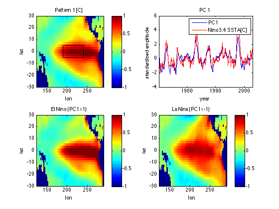
Linearity
% Compare patterns for strong positive and negative polarities of PC1, each
% scaled to an equivalent PC1 = 1 pattern.

ElNino = (PC1 > 1);
LaNina = (PC1 < -1);

SSTA_ElNino = mean(SST(:,ElNino'),2)/mean(PC1(ElNino));
SSTA_LaNina = mean(SST(:,LaNina'),2)/mean(PC1(LaNina));

UposPC1 = nan(ns,1);
UposPC1(~land,:) = SSTA_ElNino;
UposPC1 = reshape(UposPC1,nlon,nlat);  % Turn column of U into a lat/lon
                                    % matrix including nan's at land points

subplot(2,2,3)
image([lonmin lonmax],[latmin latmax],UposPC1','CDataMapping','scaled')
xlabel('lon')
ylabel('lat')
axis xy
caxis([-1 1])
colorbar
title('El Nino (PC1>1)')

UnegPC1 = nan(ns,1);
UnegPC1(~land,:) = SSTA_LaNina;
UnegPC1 = reshape(UnegPC1,nlon,nlat);  % Turn column of U into a lat/lon
                                    % matrix including nan's at land points

subplot(2,2,4)
image([lonmin lonmax],[latmin latmax],UnegPC1','CDataMapping','scaled')
xlabel('lon')
ylabel('lat')
axis xy
caxis([-1 1])
colorbar
title('La Nina (PC1<-1)')

% Slight spatial pattern nonlinearity is evident, esp. for La Nina phase.
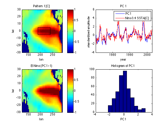
Look if PDF of PC1 is multimodal (shows clustering)
subplot(2,2,4)
hist(PC1)
xlabel('PC1')
title('Histogram of PC1')

% PDF of PC1 is slightly skewed but has a single main peak - no evidence of
% clustering
Now add plots for mode 2
U2 = reshape(Uall(:,2),nlon,nlat);  % Turn column of U into a lat/lon
                                    % matrix including nan's at land points
Ut2 = U2*s(2)/sqrt(nt-1);
Vt2 = V(:,2)*sqrt(nt-1);               % Renormalize V to have std=1

subplot(2,2,3)
image([lonmin lonmax],[latmin latmax],Ut2','CDataMapping','scaled')
xlabel('lon')
ylabel('lat')
title('Pattern 2 [C]')
caxis([-1 1])
axis xy
colorbar

subplot(2,2,4)
plot(yd,Vt2)
xlabel('year')
ylabel('standardized amplitude')
xlim([yd(1) yd(end)])
title('PC 2')

% Note patterns 1 and 2, and time series of PCs 1 and 2 are orthogonal.