PCA and rotated PCA of cities dataset in Matlab Statistics Toolbox
Illustrates principal component analysis of multicategory data Except for the rotation, this is also a worked example in the statistics toolbox.
Contents
- Load the data
- Look at the distribution of the data
- Transpose and normalize data so that each category is a different row.
- SVD of data matrix
- Plot first pattern
- Flip sign (can do due to sign ambiguity for all modes)
- Which cities score best/worst in this first pattern?
- PCA and varimax-rotated PCA with Matlab statistics toolbox functions
Load the data
  clear
  load cities
  whos  % Gives ratings, city names and rating categories
  Name              Size            Bytes  Class     Attributes

  categories        9x14              252  char
  names           329x43            28294  char
  ratings         329x9             23688  double
Look at the distribution of the data
  categories
  figure(1)
  clf
  plot(ratings)
  xlabel('City index')
  ylabel('Rating')
  legend(categories)
categories =

climate
housing
health
crime
transportation
education
arts
recreation
economics

Transpose and normalize data so that each category is a different row.
  S = ratings';
  [m,n] = size(S);
  Smean = mean(S,2)*ones(1,n);% Matrix whose rows are filled with the
                              %  mean of S for that row
  Sstd = std(S,0,2)*ones(1,n);% Matrix whose rows are filled with the
                              %  standard deviation of S for that row
  S = (S - Smean)./Sstd;      % Data is now normalized

  % Plot standardized data for Seattle

  figure(2)
  clf
  cityChar1to7 = ['Seattle';'Phoenix';'Pascago';'Washing'];
  for i= 1:4
    subplot(2,2,i)
    icity = find(strcmp(cityChar1to7(i,:),cellstr(names(:,1:7))));
    plot(S(:,icity),'x')
    title(names(icity,:))
    xlim([0 10])
    ylim([-4 4])
    xlabel('Category')
    ylabel('Standardized rating')
    if(i==1)
      text(0.2+zeros(9,1),0.2:-0.5:-3.8,categories)
    end
  end

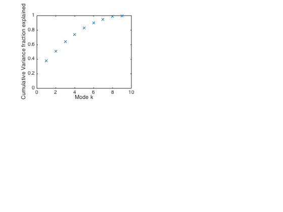
SVD of data matrix
[U,Sigma,V] = svd(S,'econ');  % Always use economy SVD option to
                       % prevent possible massive unneeded computation.
s = diag(Sigma); % Vector of singular values

% Plot cumulative variance explained by first k modes

normsqS = sum(s.^2);

figure(3)
clf
subplot(2,2,1)
plot(cumsum(s.^2)/normsqS,'x')  % Cumulative fraction of variance explained
xlabel('Mode k')
ylabel('Cumulative Variance fraction explained')
ylim([0 1])

% We see mode 1 explains 40% of the variance; all other modes are less than
% 15%.  Thus, the first pattern is a useful combination of categories.
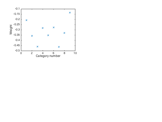
Plot first pattern
u1 = U(:,1);
figure(4)
clf
subplot(2,2,1)
plot(u1,'x')
xlabel('Category number')
ylabel('Weight')

% This is a rough average across the categories, with all categories
% having comparable negative weights.
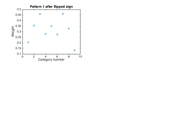
Flip sign (can do due to sign ambiguity for all modes)
Since positive scores are good, and the pattern involves all negative weights, we flip the signs of u1 and the corresponding v1 so that v1 is an indicator of 'goodness of life'
u1 = - u1;
subplot(2,2,1)
plot(u1,'x')
xlabel('Category number')
ylabel('Weight')
title('Pattern 1 after flipped sign')
Which cities score best/worst in this first pattern?
v1 = -V(:,1);  % Flip sign in v1 to correspond to flipped sign of u1
PC1 = v1/std(v1); % Standardize for easier interpretation
[PC1sort,i1sort]=sort(PC1);  % Sort PC1 from smallest to largest

iworst = i1sort(1:3);  % Indices of three cities with lowest PC1 (worst).
worst_cities = names(iworst,:)
PC1worst = PC1(iworst)

ibest = i1sort(end:-1:(end-2));  % Indices of three cities with highest PC1.
best_cities = names(ibest,:)
PC1best = PC1(ibest)

% The PC1 scores suggest much more differentiates the best cities
% (large positive PC1 = v1) from the average than for the worst cities.

% PC1 for Seattle

iSea = find(strcmp('Seattle',cellstr(names(:,1:7))));
PC1Seattle = PC1(iSea)  % PC1 positive for Seattle, i.e. high quality of life.
worst_cities =

Gadsden, AL
Dothgan, AL
Pascagoula, MS


PC1worst =

   -1.5792
   -1.5106
   -1.4811


best_cities =

New York, NY
San Francisco, CA
Los Angeles, Long Beach, CA


PC1best =

    6.7309
    4.0037
    3.9251


PC1Seattle =

    2.1581
PCA and varimax-rotated PCA with Matlab statistics toolbox functions
Note PCA assumes data matrix is n x m, the transpose of our convention
[U,SigmaV,lambda] = pca(S');

% Here, if r = min(n,m),
%  the kth element of lambda = s^2/(n-1) [r x 1] is the variance of mode k,
%  the kth column of U [m x r] is the kth pattern, with 2-norm = 1.
%  the kth column of SigmaV(:,k) [n x r] is the kth PC, normalized to
%    have variance lambda(k).

% Follow PCA with varimax rotation to try to force patterns to be
% concentrated into particular categories.  Restrict patterns to first three
% modes.  rotatefactors is a Matlab statistics toolbox function.

krot=2;
[Urot,T] = rotatefactors(U(:,1:krot)); % [m x krot]

% Expansion coefficients of rotated patterns are the
% projection of the data matrix onto these patterns.
% In this example we let the patterns carry the variance in the data

Vrot=S'*Urot;  % [n x krot] matrix of rotated expansion coeffs

figure(5)
clf

% Plot PCA pattern 1 and rotated pattern 1
% Note rotated pattern 1 is more 'localized' (more components near zero)

subplot(2,2,1)
plot(1:m,Urot(:,1),'rx',1:m,U(:,1),'bx',[0 m+1],[0 0],'k--')
legend('Rotated Mode 1','Unrotated Mode 1','Location','SouthWest')

% Calculate variance of PC1 and rotated PC1
% Note rotated PC1 cannot explain as much variance as PC1

var_PC1 = var(SigmaV(:,1))
var_rPC1 = var(Vrot(:,1))

% Plot PCA pattern 2 and rotated pattern 2

subplot(2,2,2)
plot(1:m,Urot(:,2),'mx',1:m,U(:,2),'cx',[0 m+1],[0 0],'k--')
legend('Rotated Mode 2','Unrotated Mode 2','Location','SouthWest')

% Calculate variance of PC2 and rotated PC2

var_PC2 = var(SigmaV(:,2))
var_rPC2 = var(Vrot(:,2))

% Scatterplot of data projected onto the two leading PCA patterns
% Note there is more scatter in PC1 direction, and there is no
% systematic correlation between scatter in the PC1 and PC2 dirs

subplot(2,2,3)
plot(SigmaV(:,1),SigmaV(:,2),'b.')
xlabel('Proj onto u_1')
ylabel('Proj onto u_2')
axis equal

% The 2 orthogonal modes produced by varimax rotation

subplot(2,2,4)
plot([0 T(1,1)],[0 T(2,1)],'r',[0 T(1,2)],[0 T(2,2)],'m')
legend('Rot mode 1','Rot mode 2')
xlabel('Proj onto u_1')
ylabel('Proj onto u_2')
xlim([-1 1])
axis equal
var_PC1 =

    3.4083


var_rPC1 =

    2.6275


var_PC2 =

    1.2140


var_rPC2 =

    1.9947
