Linear regression example

Analyze how temperature across the U.S. covaries
with tropical Pacific sea-surface temperature anomalies

Contents

load data

clear
load USTA;  % US monthly temperature anomaly on 5x5 degree grid
            % over U.S (NOAA GHCN3), Jan. 1970-Dec. 2002
load SSTA;  % Nino 3.4 (equatorial tropical Pacific) SSTA
whos

% Define other useful parameters

latmax = lat(1);
latmin = lat(end);
nlat = length(lat);

lonmin = lon(1);
lonmax = lon(end);
nlon = length(lon);
ns = nlat*nlon;

nyear = length(year);
nt = 12*nyear;

  Name         Size             Bytes  Class      Attributes

  SSTA       756x1               6048  double               
  TA           4-D             190080  double               
  land         5x12                60  logical              
  lat          1x5                 40  double               
  lon          1x12                96  double               
  month        1x12                96  double               
  year         1x33               264  double               
  yr         756x1               6048  double               

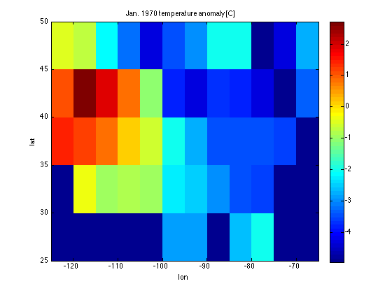
Plot a sample of the US temperature anomaly data (Jan. 1970)

TA197001 = squeeze(TA(:,:,1,1)); % 5 lats x 12 lons
image([lonmin lonmax],[latmax latmin],TA197001,'CDataMapping','scaled');
axis xy
xlabel('lon')
ylabel('lat')
title('Jan. 1970 temperature anomaly [C]')
colorbar

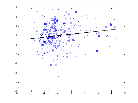
Plot a time series for the Seattle gridpoint

TAPacNW = squeeze(TA(1,1,:,:)); % 12 months x 33 years;
TAPacNW = TAPacNW(:);

yd = ones(12,1)*year + (month'-0.5)/12*ones(1,nyear);
yd = yd(:);
plot(yd,TAPacNW)
xlim([1970 2003])
xlabel('year')
ylabel('Pac NW monthly temperature anomaly')

SSTANino34 = SSTA((yr>1970)&(yr<2003));
SSTANino34 = SSTANino34 - mean(SSTANino34);

R = corrcoef(TAPacNW,SSTANino34);
R = R(2,1)   % Small but significant
sigy = std(TAPacNW);
sigx = std(SSTANino34);
plot(SSTANino34,TAPacNW,'x',SSTANino34,SSTANino34*R*sigy/sigx,'k-',1,R*sigy/sigx,'ro')

R =

    0.1455

Regression

x = SSTANino34;
y = reshape(TA,ns,nt);
y = y';
xTx = SSTANino34'*SSTANino34;
xTy = SSTANino34'*y;

a1 = xTy/xTx;
a1 = reshape(a1,nlat,nlon);

image([lonmin lonmax],[latmax latmin],a1,'CDataMapping','scaled');
axis xy
xlabel('lon')
ylabel('lat')
colorbar
title('Regression of temperature on Nino3.4 SSTA')

Multiple regression of Pac NW SST on first three PCs of Pac SST

load SSTPac
SST = PSSTA(~land,:);
SST = SST - mean(SST,2)*ones(1,nt);  % Remove any residual time-mean at each location.
[U,Sigma,V] = svds(SST,3);  % Always use 0 argument (economy SVD option) to
                       % prevent possible massive unneeded computation.
X = V./(ones(nt,1)*std(V));  % Normalize PCs to variance 1.
y = TAPacNW;

% Solve (X'X)a = X'y, where LHS is a 3x3 matrix and RHS and a are 3x1

a = (X'*X)\(X'*y);
yhat = X*a;

% Have we improved the correlation coefficient at all vs. using only PC1?

R1 = corrcoef(X(:,1),y);
R1 = R1(2,1)
R3 = corrcoef(yhat,y);
R3 = R3(2,1)

R1 =

    0.2289


R3 =

    0.2712

Published with MATLAB® R2012b