Apply cluster analysis to cities dataset

That is, cluster cities that have similar quality of life metrics.

Contents

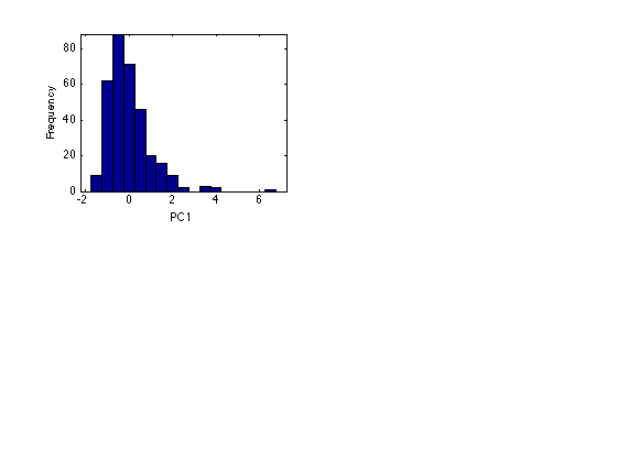
Load and standardize the data, and calculate its PCA

% Note that the data array for k-means cluster analysis in Matlab should
% have rows correspond to the n samples and columns to the m variables,

  load cities

  % Make an n x m matrix R

  R = ratings;
  [n m] = size(ratings);
  Rmean = ones(n,1)*mean(R);  % nxm matrix whose cols are filled with the
                              %  mean of S for that col
  Rstd = ones(n,1)*std(R);    % nxm matrix whose cols are filled with the
                              %  standard deviation of S for that cols
  R = (R - Rmean)./Rstd;      % Ratings data matrix R is now normalized

  %
  [U,SigmaV,lambda] = pca(R);
  PC1 = SigmaV(:,1);
  PC1 = PC1/std(PC1);  % Standardize for simplicity of interpretation
  subplot(2,2,1)
  xbin = -2:0.5:7;
  hist(PC1,xbin)
  axis tight
  xlabel('PC1')
  ylabel('Frequency')

1. Apply k-means cluster analysis to PC1 [n x 1]

Note that the clustering comes out slightly differently each time because the clusters are seeded to start, and with the 'cluster' option the seeding using a randomly selected 10% of the data for an initial clustering with which to derive the initial centroids.

  K = 4;  % Arbitrarily look for four clusters
  [ID1,ClusterCentroid1,SSE1] = kmeans(PC1,K,'start','cluster');
  SumSqErr1 = sum(SSE1)   % Sum of squared distances to centroids (error metric)

  %  Sort cities in each cluster into PC1 bins

  nbin = length(xbin);
  ClusterFreq1 = zeros(nbin,K);
  for id = 1:K
    ClusterFreq1(:,id) = hist(PC1(ID1==id),xbin);
  end

  % Plot stacked bar chart, with bar width 1
  subplot(2,2,2)
  bar(xbin,ClusterFreq1,1,'stacked')
  axis tight
  xlabel('PC1')
  ylabel('Frequency')

  %  Add text in appropriate color giving each cluster centroid
  %  This involves mapping the vector 1:K onto the rows 1:ncolors
  %  of the colormap being used by bar().

  BinFreq = hist(PC1,xbin);
  CFmax = max(BinFreq);
  ColorMap = colormap;
  ncolors = size(ColorMap,1);
  textcolor = zeros(K,3);  % RGB colors for the K clusters
  for id = 1:K
    textcolor(id,:) = ColorMap(1+round((ncolors-1)*(id-1)/(K-1)),:);
    text(3,(1-0.1*id)*CFmax,['Centroid ' num2str(id) ' = ' ...
                            num2str(0.1*round(10*ClusterCentroid1(id)))],...
         'Color',textcolor(id,:))
  end
  title('Clustering of PC1 only')

SumSqErr1 =

   40.5595

2. Apply k-means cluster analysis to full normalized dataset R [n x m]

  K = 4;  % Arbitrarily look for four clusters
  [ID2,ClusterCentroid2,SSE2] = kmeans(R,K,'start','cluster');
  SumSqErr2 = sum(SSE2)

  %  Sort cities in each cluster into PC1 bins for plotting

  nbin = length(xbin);
  ClusterFreq2 = zeros(nbin,K);
  for id = 1:K
    ClusterFreq2(:,id) = hist(PC1(ID2==id),xbin);
  end

  % Plot stacked bar chart, with bar width 1
  subplot(2,2,4)
  bar(xbin,ClusterFreq2,1,'stacked')
  axis tight
  xlabel('PC1')
  ylabel('Frequency')
  for id = 1:K
    textcolor(id,:) = ColorMap(1+round((ncolors-1)*(id-1)/(K-1)),:);
    text(3,(1-0.1*id)*CFmax,['Cluster ' num2str(id)],...
         'Color',textcolor(id,:))
  end
  title('Clustering of full normalized data matrix')

  % Plot the four cluster centroids vs. the 9 quality-of-life variables

  subplot(2,2,3)

  for id = 1:K
    plot(ClusterCentroid2(id,:),'x','Color',textcolor(id,:))
    hold on
  end

  %  Add first 3 letters of category names at top.  This is easiest if
  %  we fix the y-axis limits

  ylim([-1 3])
  for icat = 1:9
    text(icat,2.8,categories(icat,1:3),'HorizontalAlignment','center')
  end

  xlabel('Quality of Life Category')
  ylabel('Normalized value')
  title('Cluster Centroids')
  hold off

  % Panel 4 comments:
  % Now clusters mix across PC1 (expected, since other directions explain
  % a combined 60% of the variance).  Also, the clusters vary more with
  % the initial random seed, suggesting they are not very robust.

  % Panel 3 comments:
  % Mostly, the cluster centroids are different from each other in being
  % simultaneously larger or smaller in all QOL measures (i. e. along the
  % direction of pattern 1), but some ('health', 'art') are more prominent.

SumSqErr2 =

   1.8695e+03

Published with MATLAB® R2012b