4-variable Kalman estimation of ball tracking problem

Contents

First set model parameters and generate truth

u0 = -20;
w0 = 20;
r0 = 80;
z0 = 0;
g = 9.8; % gravitational acceleration
sigo = 0.001; % std of obs about truth
dt = 0.1;
N = 40; % Number of samples
t = (0:(N-1))*dt;

% Generate truth

rtrue = r0 + u0*t;
ztrue = w0*t - 0.5*g*t.^2;
ytrue = atan(ztrue./rtrue);

% Make observation vector

yo = ytrue + sigo*randn(1,N);

Kalman estimation of state vector x = [r z u v]'

% Initialize quantities to be stored at every timestep

xhat = nan(4,N);  % State vector
sigr = nan(1,N);
sigz = nan(1,N);
sigu = nan(1,N);
sigw = nan(1,N);

% Initialize estimated state and covariance matrix

uguess = -10;
vguess = 5;
xhat(:,1) = [r0 0 uguess vguess];

rvar0 = 10;
zvar0 = 1;
uvar0 = 10^2;
wvar0 = 10^2;
Chat = diag([rvar0 zvar0 uvar0 wvar0]);

% Set up time-independent matrices used in Kalman filter

Co = sigo^2;  % Covariance 'matrix' [1x1] of observations

F = [1 0 dt 0; 0 1 0 dt; 0 0 1 0; 0 0 0 1];  % Update matrix

% Time-step using Kalman filter

for n = 2:N

  % Predict

  rhat = xhat(1,n-1);
  zhat = xhat(2,n-1);
  uhat = xhat(3,n-1);
  what = xhat(4,n-1);
  xp = [rhat + uhat*dt; zhat + what*dt - 0.5*g*dt^2; ...
        uhat; what - g*dt]; % f(xhat)
  Cp = F*Chat*F';  % 2x2

  % Update

  rp = xp(1);
  zp = xp(2);
  hp = atan(zp/rp);
  H = [-zp rp 0 0]/(rp^2 + zp^2);
  K = Cp*H'/(H*Cp*H' + Co); % Use plain division since inverting 1x1 matrix
  Chat = (eye(4)-K*H)*Cp;
  xhat(:,n) = xp + K*(yo(n) - hp);
  sigr(:,n) = sqrt(Chat(1,1));  % std of rhat uncertainty at step n
  sigz(:,n) = sqrt(Chat(2,2));  % std of zhat uncertainty at step n
  sigu(:,n) = sqrt(Chat(3,3));  % std of zhat uncertainty at step n
  sigw(:,n) = sqrt(Chat(4,4));  % std of zhat uncertainty at step n
end

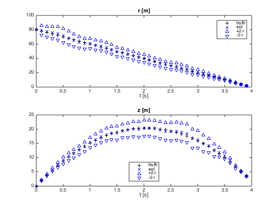
Output results

% Redefine zhat and rhat to include all times.
rhat = xhat(1,:);
zhat = xhat(2,:);

% Plot exact and estimated r, including 2-std uncertainty bounds.

figure(1)
clf
subplot(2,1,1)
plot(t,rtrue,'k+',...
     t,rhat,'bx',...
     t,rhat+2*sigr,'b^',...
     t,rhat-2*sigr,'bv')
xlabel('t [s]')
legend('truth','est','+2\sigma','-2\sigma','Location','NorthEast')
title('r [m]')

% Plot exact and estimated z, including 2-std uncertainty bounds.
subplot(2,1,2)
plot(t,ztrue,'k+',...
     t,zhat,'bx',...
     t,zhat+2*sigz,'b^',...
     t,zhat-2*sigz,'bv')
xlabel('t [s]')
legend('truth','est','+2\sigma','-2\sigma','Location','South')
title('z [m]')

Time series of angle y vs. observation

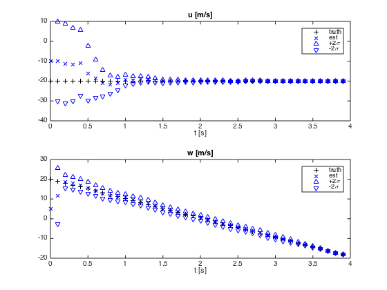
Time series of estimated velocity components

figure(2)
clf

uhat = xhat(3,:);
utrue = u0*ones(1,N);
subplot(2,1,1)
plot(t,utrue,'k+',...
     t,uhat,'bx',...
     t,uhat+2*sigu,'b^',...
     t,uhat-2*sigu,'bv')
xlabel('t [s]')
legend('truth','est','+2\sigma','-2\sigma','Location','NorthEast')
title('u [m/s]')

what = xhat(4,:);
wtrue = w0 - g*t;
subplot(2,1,2)
plot(t,wtrue,'k+',...
     t,what,'bx',...
     t,what+2*sigw,'b^',...
     t,what-2*sigw,'bv')
xlabel('t [s]')
legend('truth','est','+2\sigma','-2\sigma','Location','NorthEast')
title('w [m/s]')

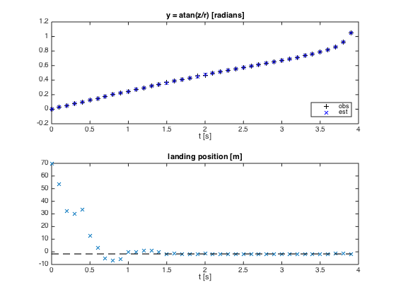
Consistency with obs, and estimated landing position

figure(3)
clf

% Check consistency of our solution with observations by comparing y vs yo

yhat = atan(zhat./rhat);
subplot(2,1,1)
plot(t,yo,'k+',t,yhat,'bx')
xlabel('t [s]')
legend('obs','est','Location','SouthEast')
title('y = atan(z/r) [radians]')

% Where will the ball land given estimated state at time step n?

subplot(2,1,2)
dtf = (what + sqrt(what.^2 + 2*g*zhat))/g;  % Time to impact
rf = rhat + uhat.*dtf; % location at impact
rftrue = r0 + 2*u0*w0/g; % true impact location
plot(t,rf,'x',t,rftrue*ones(1,N),'k--')
xlabel('t [s]')
title('landing position [m]')

Published with MATLAB® R2014b