Windowed Fourier analysis of a musical sample

We use windowed DFTs to break a short segment of Handel's Messiah into its time-varying component frequencies, which are the musical notes being sung and their overtones. This is called a spectrogram.

Contents

Load data and see what we have

  load handel %this music dataset is built into Matlab
  who
  Fs  % Sampling frequency (samples/sec)
  Ny = length(y)  % Number of samples in the segment

Your variables are:

Fs  y   


Fs =

        8192


Ny =

       73113

Plot the data

  figure(1)
  clf
  subplot(2,1,1)
  plot((1:Ny)/Fs,y);
  xlabel('Time [s]');
  ylabel('Sound pressure');
  title('Music time series');

Play the data as music

  p8 = audioplayer(y,Fs);
  playblocking(p8);

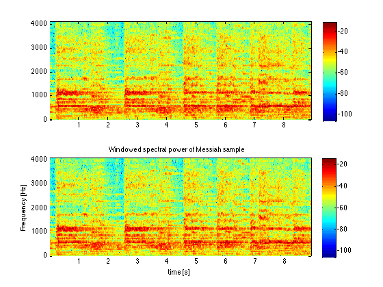
DFT power spectra using Hann window

  Nw = 256;

  j = 1:Nw;
  w = 0.5*(1-cos(2*pi*(j-1)/Nw))'; % Hanning window of length Nw:
                                   % SP toolbox: w=hanning(Nw,'periodic')
  varw = 3/8; % Mean-square value of taper function w (used to
              % renormalize power spectrum).

  % Segment the data into 'full' and 'half' windows, arrayed in columns

  nwinf = floor(Ny/Nw); % Number of 'full' windows starting each Nw samples
  nwinh = nwinf - 1;    % Number of 'half' windows (half-way between fulls)
  nwin = nwinf+nwinh;

  yw = zeros(Nw,nwin);  % Define array in which to insert windowed data
  yw(:,1:2:nwin) = reshape(y(1:nwinf*Nw),Nw,nwinf);
  yw(:,2:2:(nwin-1)) = reshape(y((1+Nw/2):(nwinf-0.5)*Nw),Nw,nwinh);

  % Taper each column (i. e. the data in each window)

  wmx = repmat(w,[1 nwin]);
  yt = wmx.*yw;

  % DFT and power spectrum of each column

  ythat = fft(yt);
  S = (abs(ythat/Nw).^2)/varw; %Windowed power spectrum
  S = S(1:Nw/2,:);  % Only keep nonnegative harmonics for plotting
  SdB = 10*log10(S); % log of spectrum in decibel-like units
  Mw = 0:(Nw/2 - 1);  % Nonnegative windowed harmonics
  fw = Fs*Mw/Nw; % "Frequencies'(inverse periods in Hz) of these harmonics
  tw = (1:nwin)*0.5*Nw/Fs; % Center time of each window

  % Plot the power spectra (log or decibel scale) vs. window time

  subplot(2,1,2)

  % Add offsets and padding so pcolor centers each cell on (tw,fw)
  % and last row/col of field is included in plots
  dfw = fw(2)-fw(1);
  dtw = tw(2)-tw(1);
  fwpad = [fw fw(end)+dfw]-0.5*dfw;
  twpad = [tw tw(end)+dtw]-0.5*dtw;
  SdBpad = SdB([1:end end],[1:end end]);
  pcolor(twpad,fwpad,SdBpad)
  xlabel('time [s]')
  ylabel('Frequency [Hz]')
  title('Windowed spectral power of Messiah sample')
  shading flat
  colorbar

Use Matlab spectrogram function to make the same plot

  [ywinhat,fw2,t2,P2] = spectrogram(y,hann(Nw,'periodic'),Nw/2,Nw,Fs);

  % Convert 1-sided power spectral density P2 (in power per Hz)
  % into two sided periodogram (in power per FFT frequency

  S2 = P2*Fs/Nw;

  SdB2 = 10*log10(S2); % Convert spectral power to decibel scale
  subplot(2,1,1)
  image(t2,fw2,SdB2,'CDataMapping','scaled')  %CDataMapping=scaled
    % uses the range of values of SdB2 to make the color scale.

  axis xy % Puts low frequencies at the bottom
  colorbar

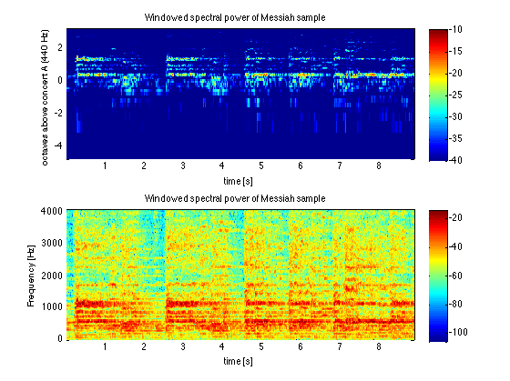
Replot with frequency in octaves from concert A = 440 Hz

  % Plot log2(freq) = octaves, but have to exclude m=1 (zero freq)

  pcolor(twpad,log2(fwpad(2:end)/440),SdBpad(2:end,:))
  caxis([-40 -10])
  xlabel('time [s]')
  ylabel('octaves above concert A (440 Hz)')
  title('Windowed spectral power of Messiah sample')
  shading flat
  colorbar

Block-average S from Nav adjacent overlapping windows, then replot

  Nav = 4; % Number of overlapping windows used for averaging spectra
  ntav = floor(nwin/Nav);
  nwininav = ntav*Nav;

  % Note use of reshape for computationally efficient block averaging
  twav = mean(reshape(tw(1:nwininav),Nav,ntav));  % Average times

  Sav = reshape(S(:,(1:nwininav)),Nw/2,Nav,ntav);
  Sav = mean(Sav,2);
  Sav = squeeze(Sav);  % Now Nw/2 x ntav
  SavdB = 10*log10(Sav);

  dtwav = twav(2)-twav(1);
  twavpad = [twav twav(end)+dtwav]-0.5*dtwav;
  SavdBpad = SavdB([1:end end],[1:end end]);
  pcolor(twavpad,log2(fwpad(2:end)/440),SavdBpad(2:end,:))
  caxis([-40 -10])
  xlabel('time [s]')
  ylabel('octaves above concert A (440 Hz)')
  title(['Windowed spectral power [dB],' int2str(Nav) '-spectrum avg'])
  shading flat
  colorbar

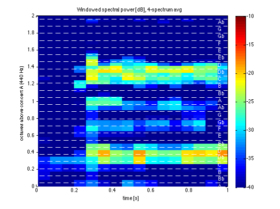
Figure 2: Zoom in on first second and two octaves and pick out notes

  figure(2)
  clf

  % Make same block-avg windowed power spectrum plot as above...
  pcolor(twav-0.5*dtwav,log2((fw(2:end)-0.5*dfw)/440),SavdB(2:end,:))
  caxis([-40 -10])
  xlabel('time [s]')
  ylabel('octaves above concert A (440 Hz)')
  title(['Windowed spectral power [dB], ' int2str(Nav) '-spectrum avg'])
  shading flat
  colorbar

  % Zoom in on the first 1 second and the two octaves above concert A

  xmin = 0;
  xmax = 1;
  xlim([xmin xmax])
  ymin = 0;
  ymax = 2;
  ylim([ymin ymax])

  % Add dotted lines showing frequency intervals centered on particular
  % notes of the musical scale.

  hold on
  plot([xmin xmax], (floor(ymin*12)+0.5:ceil(ymax*12)-0.5)'*[1 1]/12, 'w--')
  hold off
  note = ['A ';'Bb';'B ';'C ';'Db';'D ';'Eb';'E ';'F ';'Gb';'G ';'Ab'];
  text(0.95*xmax+0.05*xmin+zeros(1,24),(0:23)/12,[note;note],'Color','w')

Published with MATLAB® R2012b