Script for DFT analysis of Nino3.4 sea-surface temperature time series
Contents
- Load SST dataset and output basic statistics
- Tests for importance of endpoint discontinuities
- Calculate DFT and plot power spectrum of SST
- Demonstrate some expected theoretical properties of the DFT
- Filter out mean and first 3 harmonics of annual cycle to get SSTA
- Power spectrum and time series of SSTA
- Uncomment to save SSTA data as a .mat file for following scripts.
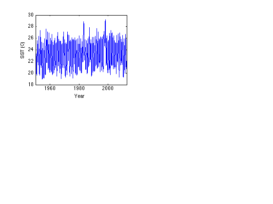
Load SST dataset and output basic statistics
  load nino

  % Plot SST
  subplot(2,2,1)
  yr = year + (month-0.5)/12; % Decimal year at center of given month
  plot(yr,SST)
  xlabel('Year')
  ylabel('SST (C)')
  xlim([year(1),year(end)+1])
  SSTmean = mean(SST)
  SSTstd = std(SST)
SSTmean =

   23.0960


SSTstd =

    2.2441
Tests for importance of endpoint discontinuities
DFT periodic extension assumption reasonable if
   |T(1)-T(N)| =  O(|T(2)-T(1)|,|T(N)-T(N-1)|
  T1_TN = SST(1) - SST(end)
                             %
  T2_T1 = SST(2) - SST(1)
  TN_TNm1 = SST(end) - SST(end-1)
T1_TN =

    1.0700


T2_T1 =

    1.0900


TN_TNm1 =

    0.8500
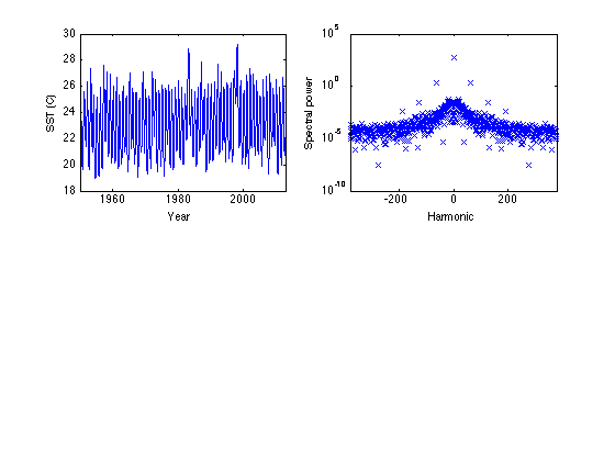
Calculate DFT and plot power spectrum of SST
  subplot(2,2,2)
  SSThat = fft(SST);
  N = length(SST);
  Nyr = N/12;
  M = [0:(N/2 - 1) -N/2:-1];
  semilogy(M,abs(SSThat/N).^2,'x')  % log scale for y due to large range
  xlim([-N/2 N/2])
  xlabel('Harmonic')
  ylabel('Spectral power')
Demonstrate some expected theoretical properties of the DFT
Show SSThat(1) related to mean(SST)
  SSThat1_over_N = SSThat(1)/N
  % Show Fourier components of harmonics +/- 1 are conjugates
  SSThat_Meq1 = SSThat(2)
  SSThat_Meqm1 = SSThat(N)
SSThat1_over_N =

   23.0960


SSThat_Meq1 =

  -4.3625e+01 + 1.3368e+02i


SSThat_Meqm1 =

  -4.3625e+01 - 1.3368e+02i
Filter out mean and first 3 harmonics of annual cycle to get SSTA
  SSTAhat = SSThat;
  filtindex = [1 + (0:3)*Nyr N+1 - (1:3)*Nyr]
  SSTAhat(filtindex) = 0;
  SSTA = real(ifft(SSTAhat));
filtindex =

     1    64   127   190   694   631   568
Power spectrum and time series of SSTA
  subplot(2,2,4)
  semilogy(M,abs(SSTAhat/N).^2,'x')
  xlim([-N/2 N/2])
  xlabel('Harmonic')
  ylabel('Spectral power')

  % IDFT to get time series of SSTA
  subplot(2,2,3)
  plot(yr,SSTA)
  ylabel('SSTA (C)')
  xlim([year(1),year(end)+1])
  SSTAstd = std(SSTA)
  SSTApower = mean(SSTA.^2) % = var(SSTA,0) or (N-1)/N * var*SSTA
  SSTAsumspectralpower = sum(abs(SSTAhat/N).^2)
SSTAstd =

    1.0707


SSTApower =

    1.1450


SSTAsumspectralpower =

    1.1450

Uncomment to save SSTA data as a .mat file for following scripts.
% save('SSTA.mat','yr','SSTA')