Nino3.4 script 2: More power spectra, lagged autocov/corr, red noise fit

Contents

Load SSTA data and plot fraction of power in various freq. ranges

  load SSTA;
  N = length(SSTA);   % Number of months in dataset
  SSTAhat = fft(SSTA);

  Nyr = N/12;         % Number of years in dataset
  M = [0:(N/2-1) -N/2:-1];  % Harmonics (note M= Nyr <-> 1 yr period)


  vartot = sum(abs(SSTAhat/N).^2)  % Total variance (using Parseval Thm)
  varsubann = 2*sum(abs(SSTAhat(2:Nyr)/N).^2)  % Subannual harmonics
     % |M|< Nyr.  Note m=1 (M=0 harmonic is ignored since it is zero,
     % because SSTA is de-meaned, and M<0 harmonics are accounted
     % for by doubling M>0 contribution.
  varfracsubann = varsubann/vartot  % Variance fraction
  varfrac2to6yr = 2*sum(abs(SSTAhat(10:30)/N).^2)/vartot % Harmonics with
     % period between 2 yrs (M = Nyr/2 = 31.5) and 6 yrs
     % (M=Nyr/6 = 10.5), i.e. 10.5 < m+1 < 31.5

vartot =

    1.1450


varsubann =

    1.0063


varfracsubann =

    0.8789


varfrac2to6yr =

    0.5421

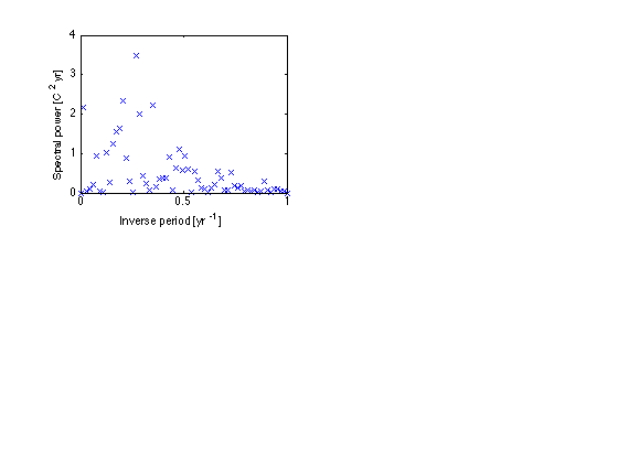
Plot power spectrum with spectral bins measured in inverse years

  subplot(2,2,1)
  plot(M/Nyr,Nyr*abs(SSTAhat/N).^2,'x')
  xlim([0 1])
  xlabel('Inverse period [yr^{-1}]')
  ylabel('Spectral power [C^2 yr]')

Calculate and plot lagged autocovariance sequence (acvs)

Three approaches

%   (1) acvsb:  Biased estimator (generally preferred)
%   (2) acvsu:  Unbiased estimator
%   (3) acvsp:  Periodically extend time series (IDFT of periodogram
%               power spectrum)
%   using Matlab xcov function.

  % acvs using 'biased' (preferred) and 'unbiased' options.

  acvsb = xcov(SSTA,'biased'); % Gives lags -(N-1) to (N-1)
  acvsb = acvsb(N:(2*N-1)); % Subset to lags 0 to (N-1)

  acvsu = xcov(SSTA,'unbiased');
  acvsu = acvsu(N:(2*N-1));

  % acvs using periodic extension - requires some gymnastics in Matlab

  % Make SSTA lag matrix with SSTAlagmx(i,j) = SSTA(i+j-1)
  % The acvs, which is the covariance between the columns of SSTAlagmx
  % can be extracted as the first row of the covariance matrix.

  SSTAlagmx = zeros(N,N);
  for lag = 0:(N-1)
    SSTAlagmx(lag+1,:) = SSTA(mod((0:(N-1))+lag,N)+1);
  end

  covmx = cov(SSTAlagmx,1); % Divide by N rather than N-1 consistent w DFT
  acvsp = covmx(:,1);

  % Verify same result from IDFT of power spectrum by showing relative
  % error of their difference is zero to rounding error.

  acvsp2 = ifft(abs(SSTAhat).^2)/N;
  relerr_acvsp = norm(acvsp-acvsp2)/norm(acvsp2)

  % Plot results

  subplot(2,2,2)
  plot(0:(N/2-1),acvsb(1:N/2),'gx',...
       0:(N/2-1),acvsu(1:N/2),'rx',...
       0:(N/2-1),acvsp(1:N/2),'bx',...
       [0 N/2],[0 0],'k--')
  xlim([0 N/2])
  xlabel('Lag [months]')
  ylabel('Autocovariance [C^2]')
  legend('biased','unbiased','periodic')

relerr_acvsp =

   5.0436e-16

Autocorrelation plot for lag < 36 months, including red-noise fit.

  maxlag = 36;
  subplot(2,2,3)
  dt = 1; % Sampling time [months]
  tau = 6.1; % Decorrelation time [months] assumed for red noise
  p = 0:(maxlag-1);  % Vector of lags
  plot(p,acvsu(p+1)/acvsu(1),'bx',...
       [0 maxlag],exp(-1)*[1 1],'g--',...
       p,exp(-p*dt/tau),'r-',...
       [0 maxlag],[0 0],'k--')
  xlabel('Lag [months]')
  ylabel('Autocorrelation (biased estimator)')
  xlim([0 maxlag])
  legend('SSTA','1/e','red noise')

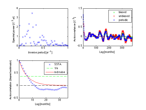
Add a red noise fit to power spectrum scaled to the total variance vartot

  subplot(2,2,1)
  hold on

  R = 1/tau; % Decorrelation rate (inverse months)
  omM = 2*pi*M/N; % Angular frequency (inverse months)
  dom = 2*pi/N;
  ps_red = (vartot/pi)*dom*R./(R^2 + omM.^2);
  plot(M(1:N/2)/Nyr,Nyr*ps_red(1:N/2),'r--')
  hold off

Published with MATLAB® R2012b