Nino3.4 Script 3: Windowed Fourier Analysis
Contents
- Plot sea-surface temperature anomaly
- Show some Hann windows
- Plot power spectrum for each window
- Focus on subannual period
- Average the spectra across windows in subannual range
- Replot using inverse period [yr^-1] as horizontal scale
- Add nino2 red noise fit
- Display as a one-sided spectrum
- Use of SP toolbox function pwelch for spectral analysis
- Fix up pwelch to match and extend our approach:
- Add red noise fit and confidence bounds
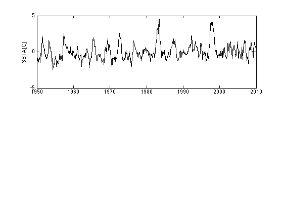
Plot sea-surface temperature anomaly
  load SSTA;   % loads decimal year yr and Nino3.4 SSTA [C].
  vartot = mean(SSTA.^2);

  Nwyr = 20; % Window length in years (User-modifiable-try 10 or 30)

  figure(1)
  clf
  subplot(2,1,1)
  plot(yr,SSTA,'k')
  ylabel('SSTA [C]')
  xlim([1950 2010])
  ylim([-5 5])
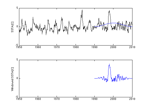
Show some Hann windows
you'll need to hit a key after the pause after each pass thru the loop
  Nw = 12*Nwyr;  % Window length in months
  Nwyr2 = Nwyr/2;  % Half-window length
  nwin = floor((yr(end)-yr(1))/Nwyr2)-1;  % Number of half-overlapping
                                          % windows of Nwyr2 yrs used
  t = 1:Nw;
  w = 0.5*(1-cos(2*pi*(t-1)/Nw))'; % Hann window of length Nw;
  varw = 3/8; % Mean-square value of taper function w (used to
              % renormalize power spectrum).

  icolor = 'rmgcb';  % Colors used for different window periods
  SSTAw = zeros(Nw,nwin);  % Windowed and tapered SSTA

  for iw = 1:nwin

    ioff = (iw-1)*Nw/2;  % Index offset
    subplot(2,1,1)
    iwc = mod(iw-1,5)+1;  % Cycle through the 5 colors
    plot(yr,SSTA,'k',yr(ioff+t),w,icolor(iwc)) % Plot taper over SSTA
    ylabel('SSTA [C]')
    xlim([1950 2010])
    ylim([-5 5])
    subplot(2,1,2)
    SSTAw(:,iw) = w.*SSTA(ioff+t);
    plot(yr(ioff+t),w.*SSTA(ioff+t),icolor(iwc))
    ylabel('Windowed SSTA [C]')
    xlim([1950 2010])
    ylim([-5 5])
    pause
  end
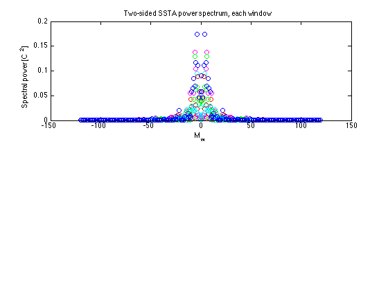
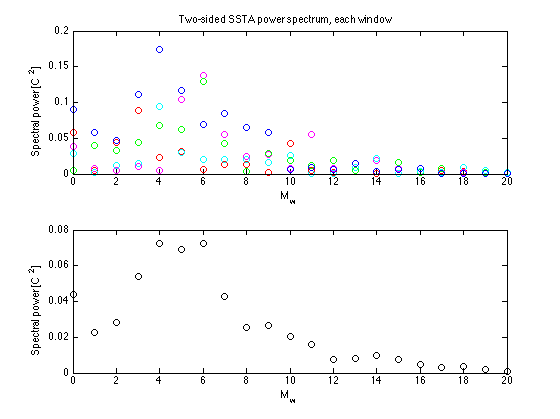
Plot power spectrum for each window
  SSTAwhat = fft(SSTAw); % Spectrum simultaneously computed
                         % column-wise for all windows
  figure(2)
  clf
  subplot(2,1,1)

  % Windowed power spectra

  Mw=[0:(Nw/2-1) -Nw/2:-1]; % Harmonics for windowed DFT
  for iw = 1:nwin
    Sw = abs(SSTAwhat/Nw).^2/varw;
    iwc = mod(iw-1,5)+1;  % Cycle through the 5 colors
    plot(Mw,abs(Sw(:,iw)),[icolor(iwc) 'o'])
    xlabel('M_w')
    ylabel('Spectral power [C^2]')
    hold on
  end
  hold off
  title('Two-sided SSTA power spectrum, each window')
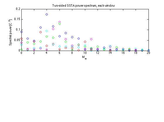
Focus on subannual period
xlim([0 Nwyr])
Average the spectra across windows in subannual range
  Swav = mean(Sw,2);
  subplot(2,1,2)
  plot(Mw,Swav,'ko')
  xlabel('M_w')
  ylabel('Spectral power [C^2]')
  xlim([0 Nwyr])
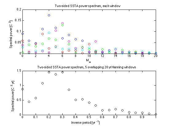
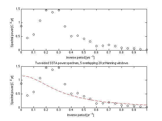
Replot using inverse period [yr^-1] as horizontal scale
  % Replot using inverse period M/Nwyr as horizontal scale instead
  % of M.  To make the horizontal integral over all inverse periods
  % (positive and negative) still equal to the power,
  % renormalize spectral power by Nwyr.

  plot(Mw/Nwyr,Swav*Nwyr,'ko')
  xlim([0 1])  % Frequency range to plot [1/yr]
  xlabel('Inverse period [yr^{-1}]')
  ylabel('Spectral power [C^2 yr]')
  title(['Two-sided SSTA power spectrum, ' int2str(nwin) ' overlapping ' ...
         int2str(Nwyr) ' yr Hanning windows'])
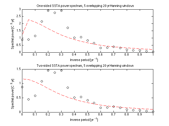
Add nino2 red noise fit
  tau = 6.1; % Decorrelation time (months)
  R = 1/tau; % Decorrelation rate (inverse months)
  omMw = 2*pi*Mw/Nw; % Angular frequency (inverse months)
  domw = 2*pi/Nw;
  hold on
  ps_red = (vartot/pi)*domw*R./(R^2 + omMw.^2);
  plot(Mw(1:Nw/2)/Nwyr,ps_red(1:Nw/2)*Nwyr,'r--')
  hold off

Display as a one-sided spectrum
(adding the power in negative harmonics to that in positive harmonics)
This is a common default in spectral analysis
  subplot(2,1,1)
  Mw_1s = [0:(Nw/2)];
  Swav_1s = [Swav(1); 2*Swav(2:Nw/2); Swav(Nw/2 + 1)]; % Col vector
  ps_red_1s = [ps_red(1) 2*ps_red(2:Nw/2) ps_red(Nw/2 + 1)]; % Row vector
  plot(Mw_1s/Nwyr,Swav_1s*Nwyr,'ko')
  hold on
  plot(Mw_1s/Nwyr,ps_red_1s*Nwyr,'r--')
  xlim([0 1])  % Frequency range to plot [1/yr]
  xlabel('Inverse period [yr^{-1}]')
  ylabel('Spectral power [C^2 yr]')
  title(['One-sided SSTA power spectrum, ' int2str(nwin) ' overlapping ' ...
         int2str(Nwyr) ' yr Hanning windows'])
  hold off
Use of SP toolbox function pwelch for spectral analysis
  subplot(2,1,1)
  pwelch(SSTA);        % Default 1-sided windowed power spectrum
                       % Window length and taper type chosen automatically
                       % There are various scaling issues
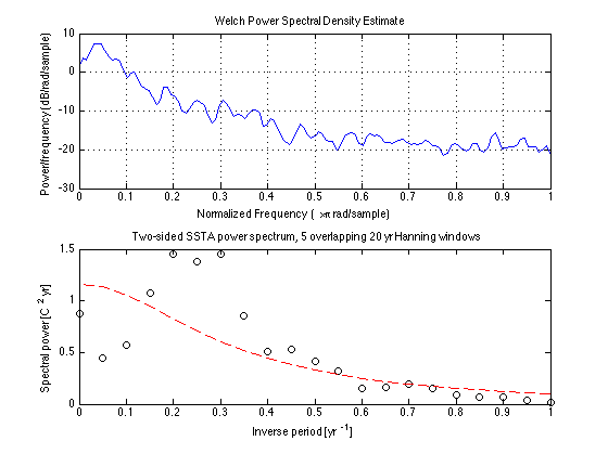
Fix up pwelch to match and extend our approach:
Use linear rather than semilogy plot
Use two-sided power spectrum rather than the default one-sided, which
 adds the power in the negative harmonics to their positive counterparts
Use Hann window of length Nw, not default Hamming window of length N/8
Calculate the windowed/tapered power spectrum at Nw frequencies
Normalize frequency to be in 1/yr instead of 1/mo
Add 95% confidence intervals
  rate = 12; % Spectrum time unit is 1 year = 12 monthly samples
  [Pxx,f,Pxxc]=pwelch(SSTA,hann(Nw),Nw/2,Nw,rate,...
      'twosided','ConfidenceLevel',0.95);

  plot(f,Pxx,'ko')
  xlim([0 1]) % Only plot inverse periods no longer than 1/yr.
  xlabel('Inverse period [yrs^{-1}]')
  ylabel('Spectral power [C^2 yr]')
  hold on
Add red noise fit and confidence bounds
  plot(Mw(1:Nw/2)/Nwyr,ps_red(1:Nw/2)*Nwyr,'r--') % %Red noise fit
  plot(f,Pxxc,'k--')  % Confidence bounds on power spectrum
  title('Two-sided SSTA power spectrum using Matlab function pwelch')
  legend('Power spectrum','Red noise fit','95% confidence bounds')
  hold off

% Note that inverse periods of 0.2-0.35/yr (3-5 yrs) are at the edge
% of being statistically significant from a red noise fit at 95% confidence
% with Nw = 20 yrs.  Shortening the window length to Nw = 10 yrs
% (try this at the beginning of the script) makes the power spectrum
% more certain but also smears the spectral power in the 3-5 yrs band
% into adjacent frequencies ('spectral leakage') so that the spectral peak
% is still only barely statistically significant.
