Mathematics

Polynomial Regression

Based on the plot, it is possible that the data can be modeled by a polynomial function

The unknown coefficients a₀, a₁, and a₂ can be computed by doing a least squares fit, which minimizes the sum of the squares of the deviations of the data from the model. There are six equations in three unknowns,

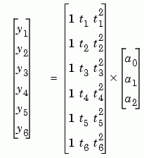
represented by the 6-by-3 matrix

X = [ones(size(t))  t  t.^2]

X = 
    1.0000         0         0
    1.0000    0.3000    0.0900
    1.0000    0.8000    0.6400
    1.0000    1.1000    1.2100
    1.0000    1.6000    2.5600
    1.0000    2.3000    5.2900

The solution is found with the backslash operator.

a = X\y

a =
    0.5318
    0.9191
  - 0.2387

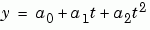
The second-order polynomial model of the data is therefore

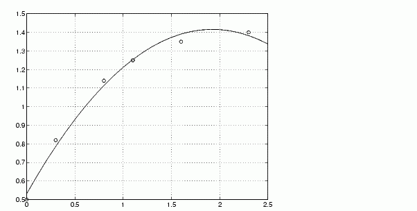
Now evaluate the model at regularly spaced points and overlay the original data in a plot.

T = (0:0.1:2.5)';
Y = [ones(size(T))  T  T.^2]*a;
plot(T,Y,'-',t,y,'o'), grid on

Clearly this fit does not perfectly approximate the data. We could either increase the order of the polynomial fit, or explore some other functional form to get a better approximation.

Regression and Curve Fitting

Linear-in-the-Parameters Regression