1.
INTRODUCTION
Model Output Statistics (MOS)
have been a useful tool for forecasters for years and have shown improving
forecast performance over time. A more recent advancement in the use of
MOS is the application of "consensus" MOS (CMOS), which is a
combination or average of MOS from two or more models. CMOS has shown
additional skill over individual MOS forecasts and has performed particularly
well in comparison with human forecasters in forecasting contests (Vislocky and
Fritsch 1997). An initial study comparing MOS and CMOS temperature
and precipitation forecasts to those of the National Weather Service (NWS)
subjective forecasts is described. MOS forecasts from the AVN (AMOS), Eta
(EMOS), MRF (MMOS), NGM (NMOS) models are included, with CMOS being a consensus
from these four models. Data from 30 locations throughout the United
States for the July 2003 - November 2003 time period are used.
Performance is analyzed at various forecast periods, by region of the U.S., and
by time/season. The results show that CMOS is competitive or superior to
human forecasts at nearly all locations.
2. DATA
Daily model and human
forecast maximum temperature (MAX-T), minimum temperature (MIN-T) and
probability of precipitation (POPs) data were gathered for 30 stations spread
across the U.S. (Figure 1), from July 1, 2003 – November 3, 2003. Forecasts were taken from the NWS, AMOS,
EMOS, MMOS, and the NMOS. An average or
“consensus” MOS (CMOS) was also calculated from the four MOS’s. Data was gathered from the 12Z forecasts
going out to 48 hours, so two MAX-T forecasts, two MIN-T forecasts, and four
12-hr POPs forecasts were gathered each day.
These were then compared with actual data to determine forecast
verification statistics.
Stations chosen for the study
are all major weather forecast offices (WFOs) and were taken from the city in
which the WFO resided. Thus,
comparisons are made at locations where forecasters are expected to have good
meteorological familiarity. The
distribution of stations across the U.S. was
* Corresponding author address: Jeffrey A.
Baars, University of Washington, Deptartment of Atmospheric Sciences, Seattle,
WA, 98195; email: jbaars@atmos.washington.edu.
intended to represent broad geographical areas of
the country.
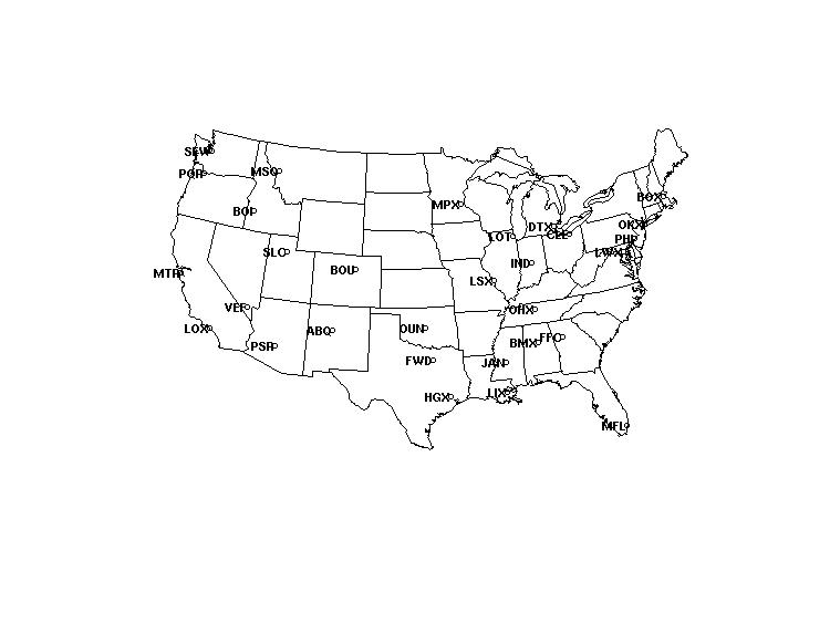
Figure 1. Map of U.S. showing station WFO ID locations used
in the study.
The definitions of MAX-T and
MIN-T followed the National Weather Service MOS definition (Jensenius et al
1993), which are a maximum temperature during the daytime and a minimum
temperature during the nighttime. Daytime
is defined as 7 AM through 7 PM local time and nighttime is defined as 7 PM
through 8 AM local time. The definition
of POPs also followed the MOS definition and were broken into two periods per
day: 00Z – 12Z and 12Z – 00Z.
Definitions of MAX-T, MIN-T, and POPs from the NWS follow similar
definitions (Chris Hill, personal communication, July 17, 2003).
While quality control
measures are implemented at the agencies from which the data was gathered,
simple range checking was performed to ensure quality of the data used in the
analysis. Temperatures below –85°F and above 140°F were removed, POPs were
checked to be in the range of 0 to 100%, and quantitative precipitation amounts
were checked to be in the range of 0.0-in to 25.0-in for a 12-hr period. On occasion forecasts and/or observation
data were not available for a given time period and these data were removed
from analysis.
3. METHODS
Each station’s data was
analyzed to determine the percentage of days when all six forecasts plus the
actual observations were available, and it was found that 85-90% of days for
each station had all data needed. There
were very few days when there was no missing observation and/or forecast data
from any station, making it not possible to remove a day entirely from analysis
when all data was not present. Missing
data was seen to occur randomly across stations and forecast types however, and
all stations or forecast types had similar amounts of missing data. Therefore, only individual missing data (and
not the corresponding entire day) were removed from the analysis.
CMOS was calculated by
averaging the four MOS model values for MAX-T, MIN-T, and POP. CMOS values were calculated only if three or
more of the four MOS’s were available and were considered “missing” otherwise.
Bias and MAE calculations
were based on forecast-observation differences, which were calculated by
subtracting observations from forecasts.
Precipitation observations were converted to binary rain/no-rain data,
which are needed for calculating Brier Scores.
Trace precipitation amounts were treated as no-rain cases.
To determine forecast skill
during periods of large temperature change, large daily temperature fluctuation
days were gathered (section 4.3). These
were defined as days when the MAX-T or MIN-T varied by +/- 10°F from the previous day. MAX-T MAE’s were calculated only for days
when the MAX-T showed this large change, and MIN-T MAE’s were only calculated
on days when the MIN-T showed the large change.
4. RESULTS
4.1 Total Statistics
Total
MAE for temperature and Brier Scores for precipitation for the six forecasts
are shown in Table 1. Total MAE scores
were calculated using all stations, both MAX-T and MIN-T’s, for all forecast
periods available. Brier Scores were
calculated using all stations and all available forecast periods. It can be seen that CMOS has the lowest
total MAE, followed by the NWS, AMOS, MMOS, EMOS, and NMOS. CMOS also has the lowest total Brier Score,
followed by AMOS, MMOS, NWS, EMOS, and NMOS.
|
Forecast |
Total
MAE (°F) |
Total
Brier Score |
|
NWS |
2.35 |
0.094 |
|
CMOS |
2.29 |
0.090 |
|
AMOS |
2.56 |
0.093 |
|
EMOS |
2.65 |
0.096 |
|
MMOS |
2.61 |
0.093 |
|
NMOS |
2.68 |
0.101 |
Table 1: Total MAE and total Brier Score for each forecast
type, July 1 2003 – November 3 2003.
Totals include data for all stations, all forecast periods, and both
MAX-T and MIN-T for temperature.
MAE’s
are notably lower than was seen by Vislocky and Fritsch (1995). This is presumably due in part to 10 more
years of model improvement. Also, the
period of record in the current study is relatively short and is biased towards
the warm season when less synoptically-perturbed weather is occurring. The National Verification Program (2003),
using data from 2003, reports similar total MAE and Brier Scores for AMOS, MMOS
and NMOS to those shown here.
4.2 Total Statistics by Forecast Period
Table
2 shows MAE by MAX-T and MIN-T for each of the forecast periods. NWS has slightly lower MAE’s than CMOS on
both the first and second period MAX-T’s, while CMOS has lower MAE’s for both
first and second period MIN-T’s. The
individual MOS’s have higher MAE’s than NWS and CMOS for all MAX-T’s and
MIN-T’s except for the second period MIN-T, where NWS has a slightly higher MAE
than AMOS. EMOS has the highest MAE’s
for MAX-T, and NMOS has the highest MAE for MIN-T.
|
Forecast |
MAX-T, pd1 (day1) |
MIN-T, pd2 (day2) |
MAX-T, pd3 (day2) |
MIN-T, pd4 (day3) |
|
NWS |
2.04 |
2.26 |
2.51 |
2.60 |
|
CMOS |
2.10 |
2.10 |
2.52 |
2.43 |
|
AMOS |
2.39 |
2.31 |
2.95 |
2.58 |
|
EMOS |
2.57 |
2.30 |
3.07 |
2.66 |
|
MMOS |
2.46 |
2.31 |
3.03 |
2.64 |
|
NMOS |
2.42 |
2.48 |
2.90 |
2.92 |
Table 2. MAE (°F) for the six models for all
stations, all time periods, July 1 2003 – November 3 2003, separated by MAX-T
and MIN-T and by forecast period.
Table
3 shows Brier Scores for each of the four 12-hr precipitation forecast
periods. It can be seen that CMOS has
the lowest (higher skill) scores for all periods.
Brier Scores are higher
during periods one and three than in periods two and four for all forecast
types. This is probably due to the
these periods corresponding to afternoons when, particular during the warm
season, hit-and-miss convective precipitation degrades forecast skill scores.
|
Forecast |
Brier Score, pd1 (day1) |
Brier Score, pd2 (day2) |
Brier Score, pd3 (day2) |
Brier Score, pd4 (day3) |
|
NWS |
0.090 |
0.088 |
0.100 |
0.098 |
|
CMOS |
0.089 |
0.083 |
0.098 |
0.093 |
|
AMOS |
0.092 |
0.086 |
0.101 |
0.092 |
|
EMOS |
0.091 |
0.088 |
0.104 |
0.101 |
|
MMOS |
0.094 |
0.086 |
0.102 |
0.092 |
|
NMOS |
0.098 |
0.091 |
0.108 |
0.106 |
Table 3. Brier
Scores for the six models for all stations, all time periods, July 1 2003 –
November 3 2003, separated by MAX-T and MIN-T and by forecast period.
4.3 Statistics During Periods of Large Temperature
Fluctuations
To determine the forecast
skill during periods of large temperature fluctuation, MAE’s were calculated on
days of a 10°F in MAX-T or MIN-T change from that of the
previous day. Results of these
calculations are shown in table 4.
|
Forecast |
Total MAE (°F) |
|
NWS |
3.64 |
|
CMOS |
3.48 |
|
AMOS |
3.63 |
|
EMOS |
3.97 |
|
MMOS |
3.68 |
|
NMOS |
4.18 |
Table 4. Total MAE
for each forecast type during periods of large temperature change (10 °F over 24-hr—see text), July
1 2003 – November 3 2003. Totals
include data for all stations, all forecast periods, with MAX-T and MIN-T
combined.
There
is about a 1.0 to 1.5°F increase in MAE’s in the
six forecast types over MAE’s for all times.
CMOS shows the lowest MAE, followed by AMOS, NWS, MMOS, EMOS, and
NMOS. This order varies slightly from
the order for all time periods, but CMOS still shows the lowest MAE. CMOS actually shows a larger decrease in MAE
over other forecast types during periods of large temperature fluctuation.
4.4 Time Series Plots of MAE and Bias
Figure 2 shows a time series
of bias for all stations for June 1, 2003 – November 3, 2003 for CMOS and
NWS. The correlation between the CMOS
bias and NWS bias is quite evident, with CMOS showing a slight negative (cool)
bias during the warm season and the NWS showing a highly correlated but
slightly lesser cool bias compared to CMOS.
In mid-September, as the season changes, this situation reverses with
CMOS having a warm bias and the NWS again correlating highly but with slightly
less warm bias. This presumably shows
the extensive use of MOS by forecasters, and it shows their knowledge of biases
within the models.
Figure 3 shows a time series of MAE for
all stations for June 1, 2003 – November 3, 2003 for CMOS and NWS. Again the two forecasts are highly
correlated. Also shown in the plot is
the mean temperature for all 30 stations.
MAE’s for both CMOS and NWS can be seen to be increasing as the
temperature decreases with the advance into fall.
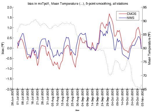
Figure 2. Time series of bias in MAX-T for period one for
all stations, July 1 2003 – November 3 2003.
5-day smoothing is performed on the data.
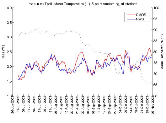
Figure 3. Time series of MAE in MAX-T for period one for all
stations, July 1 2003 – November 3 2003.
5-day smoothing is performed on the data.
4.5 Statistics by Regions of the U.S.
Figure 4 shows MAE’s for
MAX-T, period 1, for each of the 30 individual stations in the study for July
1, 2003 – November 3, 2003. The
stations are sorted by broad geographic region, starting in the West and moving
through the Inter-mountain West and Southwest, the Southern Plains, the
Southeast, the Midwest, and the Northeast (see map, Figure 1). Higher MAE’s are apparent through most of
the West, particularly at coastal cities. The Southeast generally has the
lowest MAE’s.
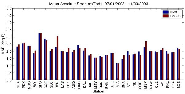 Figure
4. MAE for all stations, July 1,
2003 – November 3 2003, sorted by broad geographic region.
Figure
4. MAE for all stations, July 1,
2003 – November 3 2003, sorted by broad geographic region.
Figure
5 shows biases for MAX-T, period 1, for each of the 30 individual stations in
the study for July 1, 2003 – November 3, 2003.
The most prominent feature is positive (warm) biases in much of the
Southern Plains and Southeast and in San Francisco and Los Angeles. There are a mix of negative (cool), neutral,
and positive (warm) biases in the Midwest.
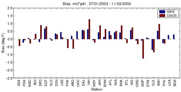
Figure 5. Bias for
all stations, July 1, 2003 – November 3 2003, sorted by broad geographic
region.
5. CONCLUSION
Results
of an initial comparison study between MOS and NWS have been shown. Similar to model ensemble averaging,
increased skill is obtained by averaging MOS from several models. Consensus Model Output Statistics (CMOS)
show equal or superior forecast performance in terms of overall MAE’s and Brier
Scores to that of the NWS and of individual MOS’s. Time series plots comparing NWS and CMOS MAE’s and biases show
the apparent extensive use of MOS by forecasters, as well as an awareness by
forecasters of seasonal biases in the models. Regional plots of MAE and bias in
temperature show the variation in forecast performance by region of the
U.S.
Future
work will include the gathering of additional data and a re-calculation of
statistics seen in the current study.
Also, statistics will be calculated during times of significant
departure from station climatology, when forecasters are expected to add more
skill to model forecasts.
6. REFERENCES
Jensenius, J.
S., Jr., J. P. Dallavalle, and S. A.
Gilbert, 1993: The MRF-based statistical guidance message. NWS
Technical Procedures Bulletin No. 411, NOAA, U.S. Dept. of Commerce, 11 pp.
Jolliffe, Ian T
and D. B. Stephenson, 2003: Forecast Verification: A Practitioner’s Guide in
Atmospheric Science. West Sussex,
England, John Wiley & Sons Ltd.
National Weather
Service National Verification Program (NVP), 2003: http://www.nws.noaa.gov/mdl/verif/,
October 27, 2003.
Vislocky, Robert
L., Fritsch, J. Michael. 1997:
Performance of an Advanced MOS System in the 1996-97 National Collegiate
Weather Forecasting Contest. Bull. Amer. Meteor. Soc.: 78,
2851-2857.
Vislocky, Robert
L., Fritsch, J. Michael. 1995a:
Improved model output statistics forecasts through model consensus. Bull. Amer. Meteor. Soc.: 76,
1157-1164.
This work was supported in part by the DoD Multidisciplinary
University Research Initiative (MURI) program administered by the Office of
Naval Research under Grant N00014-01-10745.