Presentation given at the European Geophysical Society annual meeting, Nice, France, March 26, 2001.
When I mentioned to my wife that I would be talking about Chaos, and expressed some problems with understanding what it was, she said to just take a look at my checkbook and compare my balance with that of the bank's. She of course was referring to the common definition of Chaos. Since I am going to invoke both meanings of this word, it is best that I start out with some definitions (in the first two overheads).
The existence of this new basic solution for PBL flow impacts PBL modeling, so let's look at the history of this impact --- or mostly a lack thereof.

I like to teach Ekman's solution to the Navier-Stokes equations. With Boussinesq's diffusivity constant, it is an elegant mathematical result that fits nicely into an hour lecture. All of these models listed on the slide are included in K-theory. In fact, Ekman initiated the variable K(z) studies. Also, note that Rossby & Montgomery initiated two-layer models with a mixing-length approximation for Ekman layer turbulence. This method is the basis of our PBL model at the University of Washington.


While many important details of PBL flow were discovered in the 90s, reaffirming
the nonlinear solution and the ubiquity of the Organized Large eddies (OLE),
the basic large-scale modeling situation remained the same. Meanwhile,
a revolution in large-scale PBL observations arrived in the form of global
marine surface stress data from the satellite microwave sensors.


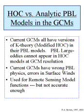
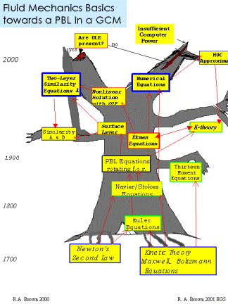
At the AMS 90th anniversary meeting I attempted to delineate the difficulties with an 'evolutionary tree' of the equations used in various PBL modeling schemes.
Signs of problems in boundary layer modelling are evident from the fact that fundamental questions have been published. When the nonlinear solution was offered it met with considerable resistance in numerical modeling circles. This is understandable --- while we start with Ekman's solution the first day, it takes most of the rest of a quarter to teach the nonlinear solution.
When GCM modelers realized this problem, observational proof of the solution
was demanded, in particular to show the existence of OLE. The response
to this request was weak in the 80s. Observations were not available except
in special campaigns. We always found OLE and it conformed to theory, but
the criticism was that we only looked in cold air outbreaks where the stratification
produced a strong energy source. I will come back to this. But first we
should look at the basic nature of the OLE to understand the problems.
Then we can address the questions about the frequency of occurrence of
OLE.
All correlations involve measurements in the Planetary Boundary Layer (PBL).
This is inherently a turbulent regime. The turbulence can only be represented
by a proper average. However, there are other organized (coherent) flows
in the PBL that are part of the mean flow on various scales and thereby
removed from 'turbulence'. Typically, these involve geophysical eddies
on scales from 100s of meters to tens of kilometers. Smaller scales can
usually be lumped in with turbulence. Large scale turbulence can be averaged and
parameterized in a 25-km footprint. This can also be done in an ad hoc
manner for OLE. But it will vary with stratification, wind speed and
sea-state. These numbers will also change as the footprint
changes, as when a Synthetic Aperture Radar (SAR) 100-meter resolution
is available the K(z) must change horizontally with position in the OLE.
The problems can be illustrated with a specific solution for a coherent
structure in the PBL from the UW solution --- the OLE. Scatterometer model
functions have typically been constructed by reference to a point source
of data --- a buoy measurement. Let's look at the fundamentals of this
measurement with a sketch of the solution with OLE (Rolls).
The rolls
fill the PBL and produce an inhomogeneity that can lead to incorrect data
comparisons. Consider measurements taken at stations A and B above. One
is in the convergent/updraft region, one near the center and downdraft
region.
The hodograph has the ratio, height/d
(Ekman depth of frictional resistance) indicated --- the top of the PBL
is at about 4-5 z/d. In
each region of the rolls the hodograph is very different. At a point it
will undulate or be steady depending on the OLE lateral movement.
In addition to atmospheric scientists,
oceanographers must be concerned about the OLE. The hodographs are the
same, and an oceanic PBL is used to illustrate the mean profile.
Note that the situation is complicated
by the fact that the analytic solution for the OLE predicts they will move
laterally with about 10% of the mean flow speed in neutral stratification.
As convective energy increases, this lateral motion goes to zero. It is
interesting that Jim Deardorff and I discussed why he wasn't getting the
OLE in his numerical PBL model in 1971. They did try to appear, but were
evanescent. Our conclusion was that, since we both had neutrally stratified,
barotropic models, the numerical model would try to establish the OLE,
but their lateral motion caused them to disappear. Unfortunately,
this conversation wasn't published --- although the results were. They
might explain why numerical models don't get OLE except in unstable stratification.
The problems in measurements
are manifest in the search for a comparison data set to establish the empirical
formulas for a satellite MF.
Consider the request for proof that the nonlinear solution with OLE is
observed. Initially, the theory was inspired by the omnipresence of cloud
streets, rows of clouds sitting on the top of the PBL as shown:
The data from the 70s consisted
of a few airplane campaigns. The argument that these weren't conclusive
proof for global PBLs was the observations were generally targeted
at cold air outbreak regions where convective energy invariably produced
rolls. The question was whether they appeared in the global ocean, that
might be nearly neutrally stratified, This question was reinforced by the
LES difficulties in obtaining OLE in neutral stratification.
The conclusions are evident as documented in this slide:


It is basically a problem of scaling in the equations and in measurement
averaging. When a model function (MF) is constructed to relate a satellite
sensor signal such as radar backscatter to a geophysical parameter such
as wind, scaling enters the correlation construction. When data is used
to establish the MF the averaging time is crucial. When a MF is used in
an oceanographic or atmospheric application, the scale must be considered.The
first procedure must be done well before the second can even be attempted.
Both have potential for serious error if the true nature of the fluid flow
involved is not fully understood. Sad to say, it often isn't.


 .
.


 The situation
today is rapidly changing because of remote sensing data. These data have
proven the ubiquitous existence of OLE. In addition they have stimulated
PBL research by demanding a global 'surface truth' value of the surface
winds in order to establish the satellite model functions.
In the 90s, observations by the SAR satellite sensors with microwave returns
from resolutions of 100-m showed OLE effects appeared in the surface wind
field (Johns Hopkins APL Technical Digest, vol 21, N 1, 2000). Subsequent
surveys showed that evidence of roll imprints on the sea surface appeared
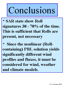
30% to 70% of the time in the North Pacific. Since the impact of the roll
wind variation on the surface must be a special case, these numbers must
represent a MINIMUM roll occurence.
The situation
today is rapidly changing because of remote sensing data. These data have
proven the ubiquitous existence of OLE. In addition they have stimulated
PBL research by demanding a global 'surface truth' value of the surface
winds in order to establish the satellite model functions.
In the 90s, observations by the SAR satellite sensors with microwave returns
from resolutions of 100-m showed OLE effects appeared in the surface wind
field (Johns Hopkins APL Technical Digest, vol 21, N 1, 2000). Subsequent
surveys showed that evidence of roll imprints on the sea surface appeared
30% to 70% of the time in the North Pacific. Since the impact of the roll
wind variation on the surface must be a special case, these numbers must
represent a MINIMUM roll occurence.
Additional information from the NASA NSCAT scatterometer
data suggested that the mean turning through the PBL was 19°,
very close to the 18°
predicted by the analytic model for neutral stratification. The angle of
turning is also observed to change as predicted for thermal wind conditions.