Mesoscale cellular convection
Boundary layer clouds exhibit a tremendous range of structures in the
mesoscale, from relatively featureless and homogeneous stratus clouds
to intricate convective patterns on with dominant scales of several
tens of kilometres. Often the clouds form mesoscale convective cells,
either open (sharp updraughts with clouds around the edges of the
cells and clear slow subsidence in the centre) or closed (slow
ascent
and clouds at the centre of the cells, with sharp downdraughts at the
edges)
form.
The nature of mesoscale cellular convection (MCC) has been the focus
of considerable attention since the 1960s. The similarity to
Benard-Rayleigh (B-R) convection are often commented upon. However,
the aspect ratios (ratio of cell width to height) can be very much
larger for atmospheric MCC. Early laboratory and numerical
model studies by Krishnamurti (J. Atmos. Sci., 32 1353-1363,
1364-1372 and 1373-1383, 1975) suggested
that
the preferred form of MCC (open or closed) depends upon whether there
is large-scale ascent (closed cells) or descent (open cells).
Determining the distribution of open and closed mesoscale
cellular
convection over the oceans
Diagnosis of cellular convection type using MODIS. From examination of
many MODIS 1km resolution images, a suitable diagnosis of open celled
convection can be obtained by examining the power contained in the
high frequency (0.2-0.5 km-1) end of the liquid water
path LWP power spectrum. Open cells generally contain
considerably
more power. In addition, the skewness of LWP (cloud+clear) also tends to be
larger in the open celled convection. The following criteria are
chosen to determine whether each 256x256 km scene has open or closed
mesoscale cellular convection:
OPEN MCC:
LWP POWER (0.2-0.5 km-1) >
250 g2 m-4
and LWP SKEWNESS > 1.8
and CLOUD FRACTION 0.1-0.75
The reason that cloud fraction alone is not a great predictior is that
many scenes contain edges between e.g. open celled convection and
clear air, or open celled convection and closed cell convection.
CLOSED MCC:
Open MCC not diagnosed
and Characteristic length scale > 10 km
The characteristic length scale is derived using the LWP
power spectrum. An example here (Fig. 1) shows three 256x256 km LWP images and
their respective power spectra below. First, an "average" wavenumber
is calculated using the LWP power spectrum as a weighting
function (see e.g. Jonker et al., J. Atmos. Sci.,
56, 801-808, 1999). The inverse of this value is a
characteristic
lengthscale (shown by the filled triangles on the abscissae)
but because it is sensitive to the power spectrum at low
freqencies, is not a good measure of the size of the mesoscale
convective
cells. However, it is useful for separating the power spectrum into
a MCC component (scales larger than the inverse average wavenumber)
and a large-scale component. We then calculate the exponent of the
power spectrum in the "intertial subrange" defined here as being
wavenumbers larger than 1.5 times the average wavenumber. The straight
dotted line is the resulting power law fit to the LWP spectrum
in the "intertial subrange". The solid circles and the dashed curves
above
and below the spectra represent the smoothed power spectrum and the
95% confidence limits on the spectrum. The point at which the
upper 95% confidence interval curve falls below the power law fit
(b and c below)
is designated as the integral scale lambda (vertical dashed lines
in Fig. 1 below).
We found that this matched
well with the characteristic length scale of the convective cells
estimated
by eye. In (a) below, the upper 95% curve never passes below the
power law fit. We found this only occurred when the eye-estimated
length scale was very small, close to the resolution of the data. We
designate the lenthscale undetermined in these cases, but note that
it is small.
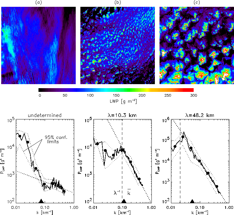
Figure 1. Three examples showing stratocumulus clouds with markedly
different convective length scales. The two-dimensional LWP
power spectra are shown below the respective images. For case (a)
the integral scale cannot be determined because it is too small. For
cases (b) and (c) the integral scales are 10.3 and 48.2 km respectively.
The characterisation process is described graphically below in
Fig. 2. Here we see a 1168x1023 km image of LWP at 1km
resolution from MODIS. The two boxed regions (both 256x256km) are
selected because they represent open and closed cellular convection.
Their power spectra are shown below (left upper panel: note that the
wavenumber has been multiplied by the power in this plot). The open
celled convection has much more power at high freqencies than the
closed cellular convection. The probability density functions for the
two
cases are shown (upper right panel). The increased skewness in the
open cellular convective case is apparent. The lower left panel shows
a plot of the power in the 0.2-0.5 km-1 range. against
skewness. The dotted lines distinguish the open celled convection (to
left and top) from non open celled convection. The lower right panel
shows the classification corresponding to the image above into
closed (red) and open (blue) cellular convection, derived using
256x256 km subscenes overlapped by 32 km. The diagnosis matches quite
well
with where the eye perceives there to be open and closed cellular
convection.
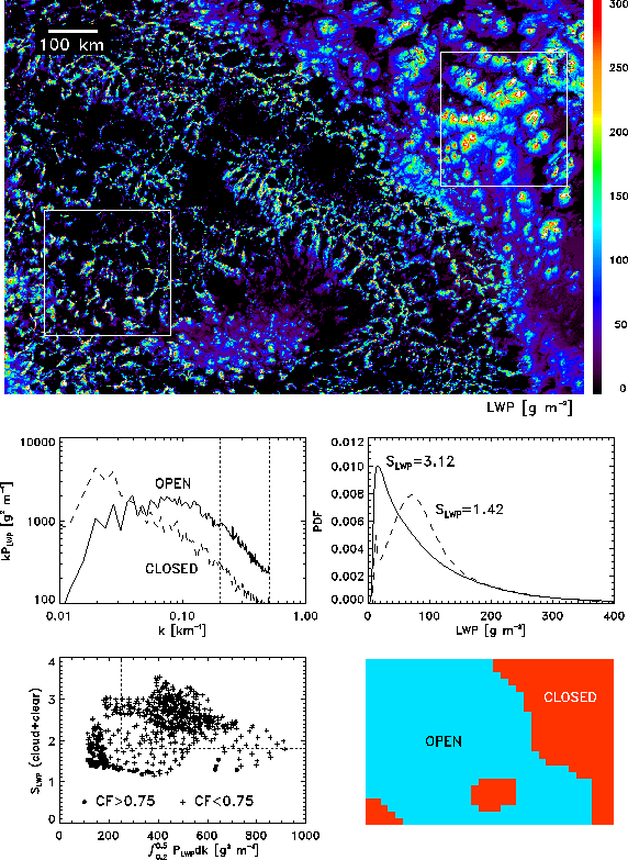
Diagnosis of open and closed cellular convection using MODIS.
Open cells are characterised by larger power at high wavenumbers and
by higher skewnesses than are found in closed cellular convection. The
method leads to a reasonably satisfactory, although by no means
perfect,
diagnosis of the locations
of open and closed cellular convection.