Diagnostic Computations Using the Command Line
This section lists operations that may be performed at the IVE command line to compute new diagnostic fields using data in the original NETCDF file.

The FIELD command is entered at the IVE command line using the format:
FIELD=expression, [new_field_name]
In response to the command, IVE evaluates the expression, creates a
new field and displays a button for the new field. If the optional
argument "newfield_name" is provided, the button will be described by
"newfield_name." If newfield_name is not provided, the expression
itself will be used for the name of the new field. (This can be
cumbersome if the expression is lengthy.) There is no limit to the
complexity of any expression, except for the recursion depth (depending
on the compiler) and for the length of the command string. The utility
breaks the expression into subexpressions, using standard mathematical
rules. Each subexpression is evaluated in the following order:
- IVE searches for the subexpression first in memory (e.g., the result of an earlier computation) and then in the data file.
- If it is not found, IVE attempts to compute the subexpression using any user-written piece of code in the routine CALC_FIELD (see Diagnostic Computations Using the Subroutine CALC_FIELD).
- The last priority is to evaluate the subexpression mathematically.
Locations flagged as missing data in the input fields are flagged
as missing data in the new diagnostic field.
Supported Operations
The expression evaluation utility supports the brackets (), {}, and []. Most mathematical standard operations are allowed. The following is a list of operations in order of ascending binding power:
- Addition and subtraction (+, -)
- Multiplication and division (*, /)
The expression A/B*C is interpreted as (A/B)*C, i.e. as in Fortran. Divisions by zero cause the flagging of the result as missing.
- Power operation (^)
Two versions of this command are implemented:
- If you enter 'field=A^2', i.e. you take the whole field to the same integer-power, then the fortran integer operation is used. This operation is also defined for A(i,j,k)<0.
- If you enter 'field=A^B' or field=A^0.5, i.e. you take the field to a real power, then the fortran real operation is used. This requires A(i,j,k)>=0. For A(i,j,k) < 0 the resulting data value is flaged as missing.
- Interpolation operation (@)
This command has maximum binding power and serves to
interpolate one field to the grid of another field. All the
aforementioned operations require fields with the same
attributes (exception see below). In case of a staggered
data-set, the fields used in an operation must first be
interpolated on the same grid. This is done with the operation
@. For instance, A@B denotes the A-field on the grid of B,
i.e. A at B.
Supported Functions
In addition, IVE supports the following mathematical functions (the
arguments must be separated by a colon):
- ABS[a]
This function returns a field containing the absolute
value of each grid point in the field 'a'.
- D[a:z]
This function returns a field containing the
derivative at each grid point in field 'a', evaluated with respect to
any Cartesian coordinate 'z'. Note: In order to compute derivatives in a
curvilinear coordinate system, you must implement the necessary code in your CALC_FIELD
subroutine (see Diagnostic
Computations Using the Subroutine CALC_FIELD).
- MAX[a:b]
This function compares the values of fields 'a'
and 'b' at each grid point and returns a field containing the maximum values.
- MIN[a:b]
This function compares the values of fields 'a'
and 'b' at each grid point and returns a field containing the minimum values.
Restrictions
- The @-operation requires that the relevant fields have the same number of dimensions, but they can have arbitrarily different attributes otherwise. All other operations may be performed using two fields with different numbers of dimensions. You can, for example, compute A*B, where A and B are dimensioned as A(15,1,10) and B(15,12). In this case it is assumed that A is uniform in the y-direction, and B is uniform in the z-direction. The operations however require that any dimensions which are greater than 1 do match, i.e. operations between A(20,30) and B(50,30) are not possible directly, but only after interpolation to the same grid, i.e. as A@B*B. It follows that a mean-array in the YZ-plane (in absence of terrain-transformations) should preferrably be defined as MEAN(1,NY,NZ), and not as MEAN(NY,NZ).
- Note that the operation A^-0.5 is not defined, but A^(-0.5) is. The same is the case for A*-0.5 and A*(-0.5).
- There are no overflow checks, i.e. you can stop the execution by asking for field=something^1000.
Compatibility with user-written functions
Command line calculations are fully compatible with user-written functions in CALC_FIELD. The user can, for instance, provide the code to calculate the potential temperature 'THETA' (see Diagnostic Computations Using the Subroutine CALC_FIELD) and perform command line calculations in terms of this new variable.
The interpolation operation is fully general and uses the user-written routines INDEX_2_PHYS, PHYS_2_INDEX and NEW_FIELD. The resulting overhead might be noticeable for three-dimensional fields. The user can write faster routines (which can take advantage of the regular structure of specific grids) within CALC_FIELD. Any such routine has priority over the standard interpolation routine, provided CALC_FIELD returns successfully.
Examples
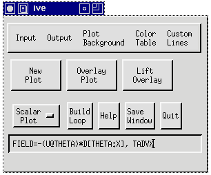
Assume that your datafile contains (or your version of CALC_FIELD
supports) the variables THETA, P, PM, U, UM, V, and W. Pictured below
is a sample FIELD command that could be used to compute the
temperature advection by the zonal wind (TADVX):

Some other examples are:
- FIELD=(9.8/300.0)*D[THETA:Z]
- Computes the square of the Brunt-Vaisala Frequency about a
reference temperature 300K.
- FIELD=U-UM or FIELD=U-10
- Evaluates the wind perturbation, or the wind with an offset.
- FIELD=THETA*[(P+PM)/1000]^0.286
- Computes the sensible temperature from the potential temperature THETA, the mean pressure PM and the perturbation pressure P.
- FIELD=(U^2+V^2+W^2)^0.5
- Computes the velocity from the wind-vector (U,V,W). Here it is assumed the components (U,V,W) are all defined on the same grid (i.e. have the same attributes). If you use a staggered dataset, see the following example.
- FIELD=(U@THETA^2+V@THETA^2+W@THETA^2)^0.5
- As previous example, but the three velocity-components are first interpolated from their (staggered) grid onto the grid defined by the variable THETA (e.g. the thermodynamic grid).
- FIELD=MAX[0:U]
- Cuts away all negative values of U.
- FIELD=(3^2+4.5^2)^0.5
- You can also use this utility as a 'pocket calculator'. The result of these operations are displayed, but not plotted.
back to index


