Time Response

No instrument responds immediately to changes in its environment. Even an unbiased instrument measuring a particular time-varying property X(t) will therefore not measure X exactly because the instrument takes a finite amount of time to respond to changes in X. Instead the instrument will record a measurement X_m(t). The rapidity of the response of the instrument can be quantified by its time constant (often given the Greek symbol tau, τ), which is a measure of the time required for the instrument to respond to a sudden change in X, as shown schematically in Figure 1.

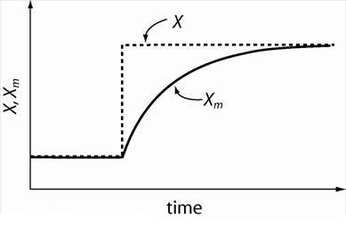
Figure 1: Schematic showing unbiased instrument response to a step change in the measured property X. The instrument indicates a measurement Xm. Before the step change, the instrument measures the true property, so X_m = X. The instrument cannot respond instantaneously to the sudden change in X, and so takes a finite amount of time to once again reach equilibrium and measure the true property X.

Why does the instrument response X_m(t) have the curved shape that it does in Fig. 1? This is related to the fundamental way in which most instruments make measurements. In the broadest sense, an instrument measures a physical property by equilibrating itself with that property. For example, wind exerts a force on a stationary anemometer. That force accelerates the anemometer until the force of friction in the system balances the force of the wind. We say then that the anemometer has equilibrated. Similarly, the mercury in a thermometer begins to expand in response to a change in temperature, and only stops responding when the temperature of the mercury is the same as the environment. The rate at which the instrumental system responds to a departure from equilibrium depends upon how far away from equilibrium the system is. The simplest analogy is the cup of initially boiling water cooling in a room. The cooling is much more rapid initially when the departure from equilibrium is greatest. When the water is quite close to room temperature, i.e. close to equilibrium, the cooling rate is much slower. This can be seen clearly in the instrumental response shown in Fig. 1. The rate at which X_m increases is greatest when X - X_m is largest (i.e. the instrument is furthest from equilibrium with its surroundings). This rate decreases as X_m becomes closer to X.

The time constant, τ

The rate at which the instrumental response X_m adjusts to come into equilibrium with the true value of X is typically linearly proportional to the deviation from equilibrium X - X_m, and acts to reduce the deviation. Therefore we can write

with the constant of proportionality being represented by the symbol τ. We can integrate Equation 1, with the boundary conditions that X-X_m = X₁ - X₀ at t = 0 (as shown in Fig. 2), to give

Thus, as t ∞, X_m X₁ and the instrument measures the true value of X, i.e. X₁. When t = τ the instrument measures a value that has reduced the initial difference X₁ - X₀ between the true and the measured value of X by a factor of 1/e (≈0.367). Thus, τ is referred to as the e-folding time, or equivalently the time constant. Small values of τ indicate that the instrument has a rapid response. For large values of τ the instrument has a slow response.

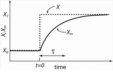
Figure 2: As in Fig. 1 but including labels indicating initial true value of property X₀  for t < 0 and the value X₁ after the step change (t > 0). Also shown is the time constant τ.

Essentially, the ideal instrument would have a time constant equal to zero, as this would mean that the instrument responds instantaneously to changes in the measurement parameter. However, in practice this is impossible. For example, the temperature sensor on a standard radiosondes package has a time response of several seconds. It is therefore not a good sensor for examining rapid thermal fluctuations in the atmosphere. The nonzero time constant for a thermometer results because the instrument itself has a finite heat capacity. It takes a finite time for the sensor to equilibrate with its environment.