Plotting a Temperature Profile on a Skew T, Log P Diagram
This file describes the procedures for creating a Skew T, Log P profile of a temperature field.

Procedures:
- It is first necessary to input a data FILE. This activates the Window/Slicer Widget (depicted below).
- At the Window/Slicer Widget, "fix" or "average" all coordinates except the vertical coordinate Adjust the fixed coordate values using the slicer bars until the appropriate horizontal location and time values for the vertical profile are displayed (as shown below).

Window/Slicer Widget
NOTE: The number of variables that you allow to vary determines the number of dimensions contained in the plot. For example, if two coordinates are "free", then IVE will create a two-dimensional plot. If you "fix" or "average" all coordinates, then a Value Info Window is activated, displaying the value of the field at the fixed point you have specified.
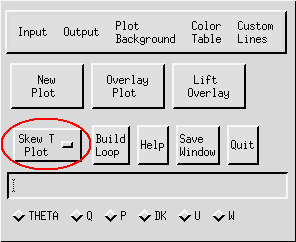
- Once you have fixed all coordinates except the vertical coordinate, the IVE Main Window is automatically changed to a one-dimensional mode. Make sure that "Skew T Plot" is displayed, unless you wish to produce a 1D plot on a linear or logarithmic scale (see Producing a 1D Scalar Plot).
 IVE Main Window in 1D Mode
- When Skew T Plot is selected, the Skew T Properties Window appears automatically (pictured below). The Skew T properties window allows you to specify the pressure component, temperature component, and dew point component (optional). Any diagnostic variable or simple mathematical computation using diagnostic variables may be entered in each box. Note that IVE assumes that the pressure component is in Pascals (N/m^2) and that temperature and dew point components are in Kelvins (see also SKEWT_COMPONENTS).
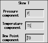
Skew T Properties Window
- Finally, when all parameters have been set, click on "New Plot" in the IVE Main Window to display the plot, or "Overlay Plot" to overlay an existing plot (see PLOT and OVERLAY PLOT).
Example:
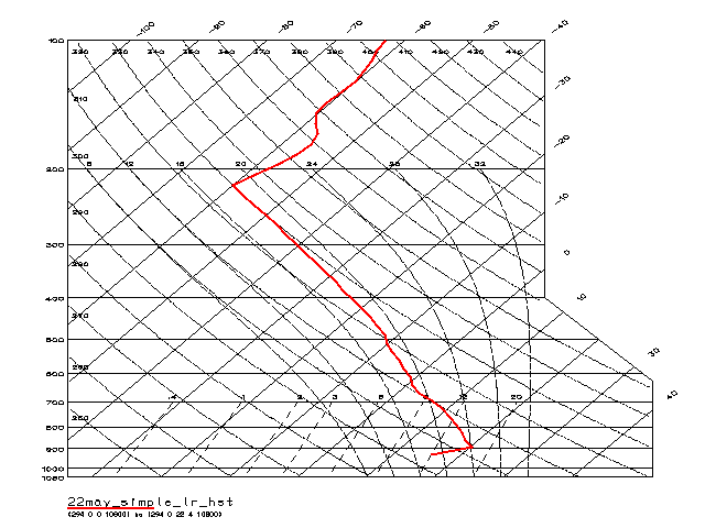
- Pictured below is a sample Skew T, Log P diagram produced by IVE:

back to index


