KwajZebra's vertical and horizontal cross-section capabilities allow the user to visualize three-dimensional structures in the data. It is necessary for all users to know how to vary the size and orientation of these cross-sections. The altitude of the horizontal cross-section in big (shown in the bottom right-hand corner) can be altered using the cursor keys. The "up" cursor key (or the letter "u") moves the altitude up to the next level. The "down" key (or the letter "d") moves the altitude down one level. The size of the horizontal cross-section can be varied by zooming in and out. To zoom in, simply click and drag the left mouse button while holding down the SHIFT button. This will draw a box around the region where the new plot will be drawn. Once the desired zoom is drawn, release the left mouse button, and the new cross-section will be created in the big window (successive cross-sections are possible). To zoom back out to the previous coordinates, simply type "b" while positioning the mouse cursor in big. To zoom out even further, it is necessary to select "Scale back to the big picture" from the "Global Options" menu (see General Setup).

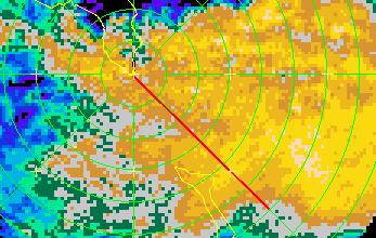
Fig. 1: The horizontal segment (in red) depicting the location of the vertical cross-sections.

The location of the vertical cross-sections is indicated in big by a line segment (shown in Fig. 1). Although this segment may be enabled/disabled from the plot with the "bounds" icon, the location of this segment remains fixed until the user specifies a new location. By altering the location of the line segment, a new orientation and size of the vertical cross-sections is specified. The new vertical cross-sections will be oriented along the vertical plane that intersects the horizontal cross-section along that line segment. To draw a new segment, simply position the mouse cursor in the big window where you want to draw the new segment. Hold the middle mouse button down while dragging the mouse to the other end of the segment, then release. The coordinate location where the mouse button was first clicked then becomes the left edge of xsect windows, and the coordinate location where the middle mouse button was released becomes the right endpoint. Once this is completed, a new segment is drawn in big, and vertical cross-sections are computed for xsect and xsect2.

The plot type, contour thickness, and contour interval may be tuned by the user to produce clear, readable plots. Three plot representation types are available: (1)raster, (2)line contour, and (3)filled contour. Any of these fields may be selected by clicking on the icon with the middle mouse button and selecting the desired representation. By selecting raster, the field appears as an image consisting of color-coded pixels. This representation is least subject to interpolation and contouring errors; however, a raster plot will ALWAYS hide all fields that are below it in the overlay stack. Both line contour and filled contour plots use a simple scheme to interpolate the data field to a Zebra grid for drawing iso-lines. Filled contour plots may partially or totally hide the displayed fields that are underneath them in the overlay stack, whereas line contours hide very little. Thus, it is good practice to display the fields on top of the stack as line contours and the fields at the bottom of the stack as filled contours or raster. The contour step may be specified using the "Overlay Options" menu (see General Setup). From this menu, select "Adjust Limits." This activates the Center/Step menu, which allows you to specify the center value (which will be assigned to the middle color in the color table), and the range of values assigned to each color. For example, consider a simple color table consisting of three colors: green, red, and yellow. If we specify a center value of 30 dBZ and a step value of 5 dBZ, then the center color in the table (in this case red) will be used to display all data values between 27.5 and 32.5 dBZ. Similarly, yellow will be used to display values between 22.5 to 27.5 dBZ, and green will indicate 32.5 to 37.5 dBZ.

KwajZebra { General | Time | Fields | Functions | Movies }

Scientific contact: Professor Sandra Yuter, Project Science Coordinator